
Net-to-gross, and the architecture behind it
The same NTG can come from a channel axis or a lobe. Place wells, type their NTG, and see which architectures fit, and where they disagree.
Synthetic demonstration data.
The lab

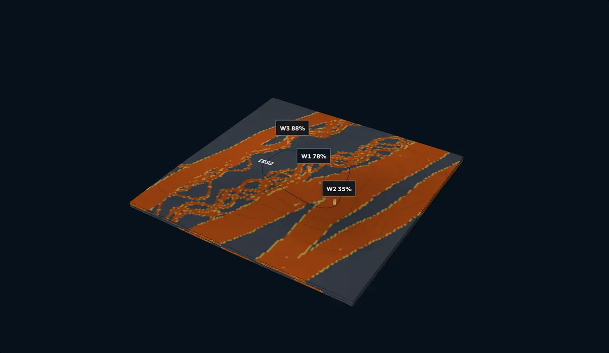
Click the map to open the 3D block
W1
NTG %. Blank where the well stops short.
Wells
Turn on Place wells, then click the map.
Which architecture fits?
Type an NTG at a well to rank the architectures.
How to read it
Each architecture against the best: how much less readily it produces your values, alone and in pairs. Within 3 times the best it fits; 3 to 20 times, possible; 20 to 150, unlikely; beyond, very unlikely (Kass and Raftery's steps).
Slice the block
Facies, zone 1. Contours: depth to top, ft.
Illustrative prospectivity, not a drilling recommendation. Share of seeded realizations, each honouring every well, that hit the target.
Confined slope channel complex, anticline, formed after deposition. Facies, zone 1. Grid: 1 mi.
Synthetic demonstration data: all datasets shown were built solely for demonstration purposes and are not client data.
Loading the lab.
Element dimensions Published defaults
Why a paleohigh matters. Over a high that grew during deposition, sands thin and shale out on the crest and thicken into the lows, so the high decides where the reservoir is. The lab honours the paleohigh when you choose Paleohigh during deposition (reefs and shoals excepted). An illustration, not a prediction for any real field.
NTG at the wells
Zone 1Type an NTG at a well.
Same wells, every architecture
Each honours every well in zone 1. Pick one.
The architectures
Nineteen, in six settings: geometry, sizes, an analogue and sources for each.
Fluvial
Braided channel belt Fluvial Compound bars and braided channels in a wide belt
Geometry
Channels and compound bars migrate across a braided belt and amalgamate. Mobile-channel belts are mainly the deposits of braided and low-sinuosity rivers, and in the rock record they can be more than 0.62 mi1 km thick and 808 mi1,300 km wide (Gibling 2006). One large mid-channel bar on the Jamuna River is about 1.86 mi3 km long, 0.62 mi1 km wide and 39 ft12 m high, grown by dunes stacking on its stoss and top and by accretion on its margins (Best et al. 2003). Bar thickness gives the channel’s maximum depth (Bridge and Tye 2000). The lab draws bars at that documented size by default and cuts them with low-sinuosity channels.
Facies
Braided channel fill, compound braid bars, finer bar tops and bar tails, mud-filled abandoned channels, and floodplain mud beyond the belt. Compound bars are three to seven sets of large-scale inclined strata, one per unit bar; their upstream and medial parts barely change grain size upward, while their downstream and lateral margins fine up (Lunt and Bridge 2004). On the South Saskatchewan River, facies vary as much within one bar as between bars (Sambrook Smith et al. 2006). The lab counts channel fill 92% net, bars 85% and bar tops 50%.
NTG behaviour
High and connected inside the belt, with mud only in abandoned channels and thin bar tops; it drops to floodplain mud at the belt edge. Wells inside one belt agree; a well beside it can read near zero.
Modern analogue
Jamuna River, Bangladesh. A sandy braided river whose mid-channel bar grew from stalled, amalgamated dunes, surveyed over 29 months (Best et al. 2003). South Saskatchewan River, Canada. Sandy unit and compound bars imaged with ground-penetrating radar (Sambrook Smith et al. 2006).
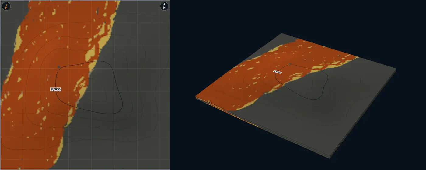
- Braided channel fill
- Compound braid bar
- Bar top and bar tail
- Abandoned-channel fill
- Floodplain mudstone
| Size | Default | Published | From |
|---|---|---|---|
| Channel-belt width | 3.11 mi5 km | Lab setting, no compiled range | – |
| Braid-bar length | 1.86 mi3 km | One documented example, 1.86 mi3 km | Best et al. (2003) |
| Braid-bar width | 0.62 mi1 km | One documented example, 0.62 mi1 km | Best et al. (2003) |
| Braid-bar thickness | 39 ft12 m | One documented example, 39 ft12 m | Best et al. (2003) |
| Channel width | 985 ft300 m | Lab setting, no compiled range | – |
| Channel thickness | 16 ft5 m | Lab setting, no compiled range | – |
| Paleoflow spread | 8° | Lab setting, no compiled range | – |
Sources for this architecture
Gibling (2006)
Gibling, M. R., 2006, Width and Thickness of Fluvial Channel Bodies and Valley Fills in the Geological Record: A Literature Compilation and Classification: Journal of Sedimentary Research, v. 76, no. 5, p. 731–770. doi:10.2110/jsr.2006.060 (opens in a new tab)
Best et al. (2003)
Best, J. L., Ashworth, P. J., Bristow, C. S., and Roden, J., 2003, Three-Dimensional Sedimentary Architecture of a Large, Mid-Channel Sand Braid Bar, Jamuna River, Bangladesh: Journal of Sedimentary Research, v. 73, no. 4, p. 516–530. doi:10.1306/010603730516 (opens in a new tab)
Bridge and Tye (2000)
Bridge, J. S., and Tye, R. S., 2000, Interpreting the Dimensions of Ancient Fluvial Channel Bars, Channels, and Channel Belts from Wireline-Logs and Cores: AAPG Bulletin, v. 84, no. 8, p. 1205–1228. doi:10.1306/A9673C84-1738-11D7-8645000102C1865D (opens in a new tab)
Lunt and Bridge (2004)
Lunt, I. A., and Bridge, J. S., 2004, Evolution and deposits of a gravelly braid bar, Sagavanirktok River, Alaska: Sedimentology, v. 51, no. 3, p. 415–432. doi:10.1111/j.1365-3091.2004.00628.x (opens in a new tab)
Sambrook Smith et al. (2006)
Sambrook Smith, G. H., Ashworth, P. J., Best, J. L., Woodward, J., and Simpson, C. J., 2006, The sedimentology and alluvial architecture of the sandy braided South Saskatchewan River, Canada: Sedimentology, v. 53, no. 2, p. 413–434. doi:10.1111/j.1365-3091.2005.00769.x (opens in a new tab)
Meandering point-bar belt Fluvial Point bars swept across a meander belt
Geometry
One sinuous channel migrates across its belt, leaving point bars on the inner banks of its bends; bends that are cut off fill with mud. In modern meandering rivers more sinuous than 1.7, bankfull width = 6.8 × depth1.54 (Leeder 1973), which gives width-to-depth ratios of about 10 for a 6.6 ft2 m deep channel and about 49 for a 125 ft38 m deep one. Meandering river bodies in the rock record are less than 125 ft38 m thick and less than 9.32 mi15 km wide (Gibling 2006). A point bar is about as thick as its channel was deep (Bridge and Tye 2000).
Facies
Lower point bar (channel lag and cross-bedded sand), upper point bar (finer, inclined heterolithic strata), levees and crevasse splays, abandoned-channel mud plugs, floodplain mud. On the Beatton River each point bar starts as a coarse platform beside the migrating bend and is capped by a scroll bar of fine sediment that becomes a floodplain ridge; about half the floodplain sediment is suspended load (Nanson 1980). The lab counts the lower point bar 90% net, the upper 60%, levees 28% and mud plugs 12%.
NTG behaviour
Every point bar fines up, so NTG falls toward the top of each storey. Sand follows the belts; mud plugs in cut-off bends cross them and can split a belt into compartments. Wells in one belt agree; wells between belts read floodplain mud.
Modern analogue
Beatton River, British Columbia. A meandering river whose point bars and scroll bars were mapped and dated; surfaces younger than 50 years build fastest (Nanson 1980).
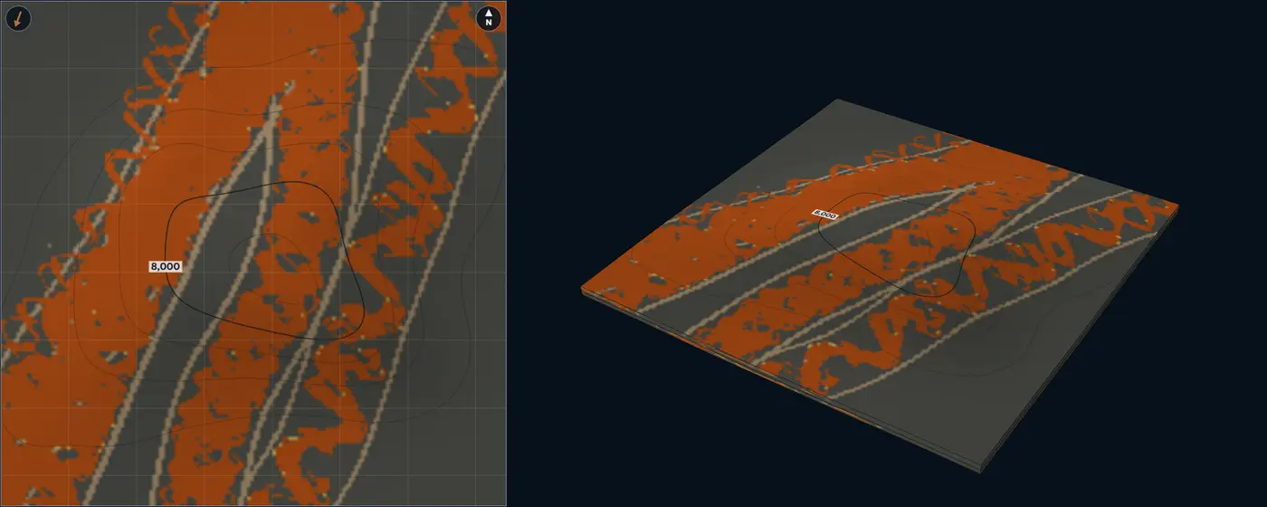
- Lower point bar
- Upper point bar
- Crevasse splay
- Levee and overbank
- Abandoned-channel fill
- Floodplain mudstone
| Size | Default | Published | From |
|---|---|---|---|
| Channel depth | 26 ft8 m | up to 125 ft38 m | Gibling (2006) |
| Channel width | 560 ft170 m | Lab setting, no compiled range | – |
| Sinuosity | 2 | 1.7 or more | Leeder (1973) |
| Meander-belt width | 0.93 mi1.5 km | up to 9.32 mi15 km | Gibling (2006) |
| Paleoflow spread | 10° | Lab setting, no compiled range | – |
| Width / depth | 21.3 | 10 to 50 | Leeder (1973) |
Sources for this architecture
Leeder (1973)
Leeder, M. R., 1973, Fluviatile fining-upwards cycles and the magnitude of palaeochannels: Geological Magazine, v. 110, no. 3, p. 265–276. doi:10.1017/S0016756800036098 (opens in a new tab)
Gibling (2006)
Gibling, M. R., 2006, Width and Thickness of Fluvial Channel Bodies and Valley Fills in the Geological Record: A Literature Compilation and Classification: Journal of Sedimentary Research, v. 76, no. 5, p. 731–770. doi:10.2110/jsr.2006.060 (opens in a new tab)
Bridge and Tye (2000)
Bridge, J. S., and Tye, R. S., 2000, Interpreting the Dimensions of Ancient Fluvial Channel Bars, Channels, and Channel Belts from Wireline-Logs and Cores: AAPG Bulletin, v. 84, no. 8, p. 1205–1228. doi:10.1306/A9673C84-1738-11D7-8645000102C1865D (opens in a new tab)
Nanson (1980)
Nanson, G. C., 1980, Point bar and floodplain formation of the meandering Beatton River, northeastern British Columbia, Canada: Sedimentology, v. 27, no. 1, p. 3–29. doi:10.1111/j.1365-3091.1980.tb01155.x (opens in a new tab)
Anastomosing ribbon channels Fluvial Stable ribbon channels in floodplain and wetland mud
Geometry
Several stable, low-slope channels split and rejoin around floodbasins. Their deposits are ribbons: Gibling (2006) classes channel bodies less than 5 times wider than thick as narrow ribbons and 5 to 15 times as broad ribbons, a narrow form that commonly reflects bank resistance and rapid filling. The channels are narrow and deep, straight to sinuous, with banks held by roots, so they aggrade in place rather than migrate (Smith and Smith 1980). In the Cretaceous Dakota Formation, Utah, anastomosed ribbon bodies are 3.3 to 30 ft1 to 9 m thick and 49 to 525 ft15 to 160 m wide, many of them coeval (Kirschbaum and McCabe 1992). New channels often reoccupy old courses, stacking ribbon on ribbon (Makaske et al. 2002).
Facies
Ribbon channel fill, levees, crevasse splays, and floodplain and wetland mud. The coarsest sediment sits in the channels, on the levees and in proximal splays; silt and clay settle on the rest of the floodplain (Nadon 1994). On the upper Columbia River, levees aggrade up to four times faster than floodbasins (Makaske et al. 2002). The lab counts ribbon fill 88% net, splays 55% and levees 28%.
NTG behaviour
Low overall. The sand sits in narrow ribbons, so a well rarely hits one, and two wells a few hundred metres apart seldom share a ribbon unless it runs between them.
Modern analogue
Upper Columbia River, British Columbia. Low-sinuosity, stable channels in a valley 74.6 by 0.93 mi120 by 1.5 km, aggrading about 2 ft0.6 m per 100 years over the past 2,500 years (Smith 1983); anastomosing for at least 2,700 years, with at least nine channels formed in one cross-valley transect in the past 3,000 years, each lasting about 800 to 3,000 years (Makaske et al. 2002). Valleys near Banff, Alberta. Three anastomosed reaches upstream of alluvial fans that raised the base level (Smith and Smith 1980).
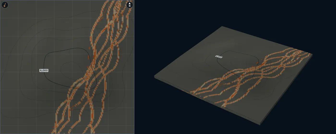
- Ribbon channel fill
- Crevasse splay
- Levee and overbank
- Floodplain mudstone
| Size | Default | Published | From |
|---|---|---|---|
| Ribbon width | 150 ft45 m | 49 to 525 ft15 to 160 m | Kirschbaum and McCabe (1992) |
| Ribbon thickness | 11 ft3.5 m | 3.3 to 30 ft1 to 9 m | Kirschbaum and McCabe (1992) |
| Levee width | 490 ft150 m | Lab setting, no compiled range | – |
| Crevasse-splay length | 2,625 ft800 m | Lab setting, no compiled range | – |
| Paleoflow spread | 10° | Lab setting, no compiled range | – |
| Width / thickness | 12.9 | 1 to 15 | Gibling (2006) |
Sources for this architecture
Gibling (2006)
Gibling, M. R., 2006, Width and Thickness of Fluvial Channel Bodies and Valley Fills in the Geological Record: A Literature Compilation and Classification: Journal of Sedimentary Research, v. 76, no. 5, p. 731–770. doi:10.2110/jsr.2006.060 (opens in a new tab)
Smith and Smith (1980)
Smith, D. G., and Smith, N. D., 1980, Sedimentation in anastomosed river systems; examples from alluvial valleys near Banff, Alberta: Journal of Sedimentary Research, v. 50, no. 1, p. 157–164. doi:10.1306/212F7991-2B24-11D7-8648000102C1865D (opens in a new tab)
Kirschbaum and McCabe (1992)
Kirschbaum, M. A., and McCabe, P. J., 1992, Controls on the accumulation of coal and on the development of anastomosed fluvial systems in the Cretaceous Dakota Formation of southern Utah: Sedimentology, v. 39, no. 4, p. 581–598. doi:10.1111/j.1365-3091.1992.tb02138.x (opens in a new tab)
Makaske et al. (2002)
Makaske, B., Smith, D. G., and Berendsen, H. J. A., 2002, Avulsions, channel evolution and floodplain sedimentation rates of the anastomosing upper Columbia River, British Columbia, Canada: Sedimentology, v. 49, no. 5, p. 1049–1071. doi:10.1046/j.1365-3091.2002.00489.x (opens in a new tab)
Nadon (1994)
Nadon, G. C., 1994, The genesis and recognition of anastomosed fluvial deposits; data from the St. Mary River Formation, southwestern Alberta, Canada: Journal of Sedimentary Research, v. 64, no. 4b, p. 451–463. doi:10.1306/D4267FE1-2B26-11D7-8648000102C1865D (opens in a new tab)
Smith (1983)
Smith, D. G., 1983, Anastomosed fluvial deposits: modern examples from Western Canada: in Modern and Ancient Fluvial Systems: International Association of Sedimentologists Special Publication 6, p. 155–168. doi:10.1002/9781444303773.ch12 (opens in a new tab)
Delta front and shallow marine
River-dominated delta front Shallow marine Delta-front lobe: distributaries, mouth bars, clinoforms
Geometry
The river mouth sits on the up-flow side and the delta-front lobe spreads from it, its proximal front sandier than its distal front. Distributaries bifurcate around mouth bars and end in bars at their tips. Each cycle coarsens up: heterolithic delta-front foresets as high as the clinoform, a mouth bar on top of them, and often the distributary channel that fed it. Later cycles sit higher and farther basinward as the delta builds out. Clinoforms span 3.3 ft1 m to 6.21 mi10 km in height, delta-scale ones are the smallest kind, and sand-prone delta foresets dip 0.1 to 2.7 degrees (Patruno et al. 2015). Distributary channels are under 0.62 mi1 km wide and about 100 times wider than thick on average (Reynolds 1999); they narrow and shorten at each bifurcation, because each mouth bar forms at a distance set by the outflow jet’s momentum (Edmonds and Slingerland 2007). A mixed-process mouth-bar complex in Alberta is up to 26 ft8 m thick, covers about 23 mi²60 km² and is built of kilometre-scale bar elements (Ainsworth et al. 2016); mouth bars are comparable in area to small fields (Reynolds 1999).
Facies
Distributary channel fill, mouth bar, heterolithic delta front and prodelta mud. Channels, bars and frontal splays sit near the distributary mouth, and storm-reworked sands spread away from it (Gani and Bhattacharya 2007). The lab counts channel fill 90% net, the mouth-bar core 84%, the distal bar 62%, the proximal front 48% and the distal front 28%. Wave-dominated coasts are the shoreface type.
NTG behaviour
Coarsening-up columns: the top of each cycle is sandy and its base heterolithic, so NTG depends on how many bar tops a zone holds and on the zone’s thickness against the clinoform height. Sand thins and fines basinward to prodelta mud.
Modern analogue
Mississippi bird-foot delta. The river-dominated end: long distributaries with their mouth bars strung along them. Wax Lake Delta, Louisiana. A lobate river-dominated delta of bifurcating channels. Growing since 1973; its distributary channels cut down by up to 40% of their flow depth by 1999 and widened 11% from 1991 to 2009 (Shaw et al. 2013).
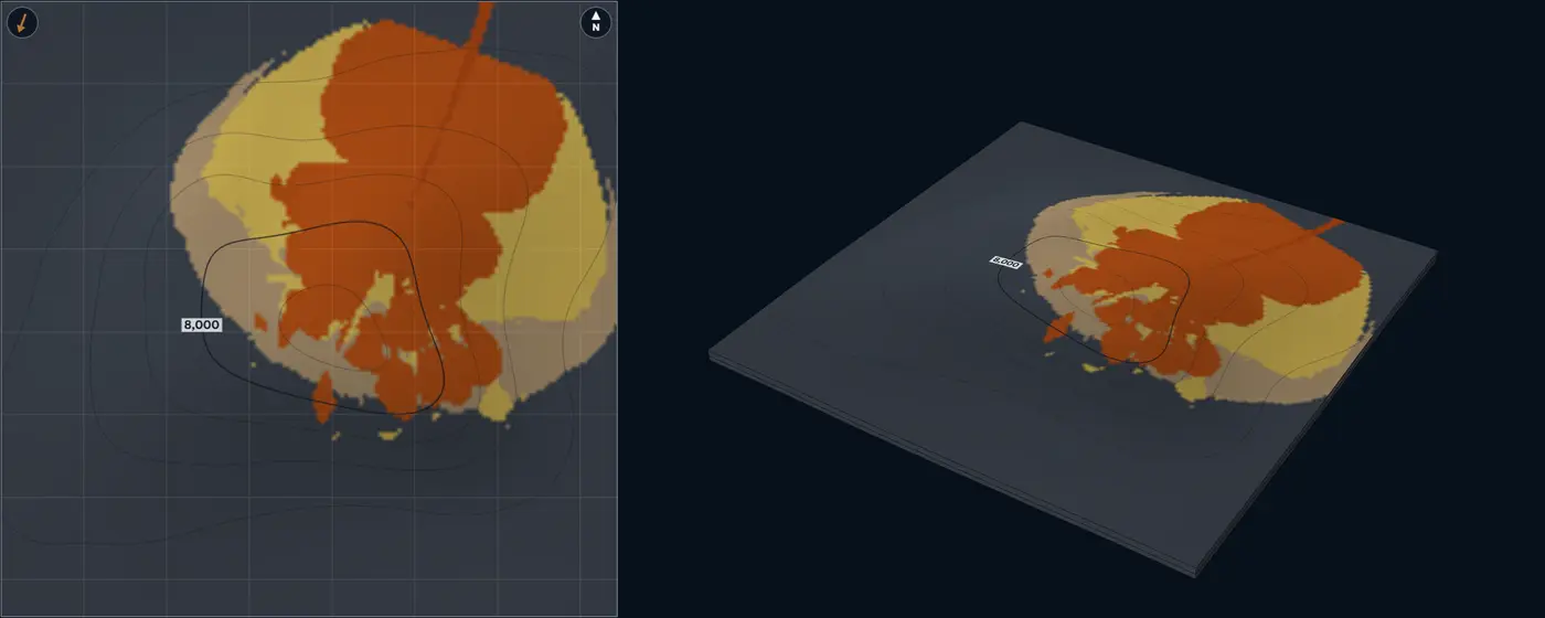
- Distributary channel
- Mouth-bar core
- Distal mouth bar
- Distal delta front and prodelta
- Mudstone and shale
| Size | Default | Published | From |
|---|---|---|---|
| Distributary channel width | 820 ft250 m | up to 3,280 ft1,000 m | Reynolds (1999) |
| Distributary channel thickness | 13 ft4 m | Lab setting, no compiled range | – |
| Mouth-bar length | 1.86 mi3 km | 0.62 to 6.21 mi1 to 10 km | Ainsworth et al. (2016); Reynolds (1999) |
| Mouth-bar width | 1.24 mi2 km | 0.62 to 6.21 mi1 to 10 km | Ainsworth et al. (2016) |
| Mouth-bar thickness | 16 ft5 m | up to 26 ft8 m | Ainsworth et al. (2016) |
| Delta-lobe length | 4.97 mi8 km | Lab setting, no compiled range | – |
| Delta-front clinoform height | 33 ft10 m | 3.3 to 195 ft1 to 60 m | Patruno et al. (2015) |
| Paleoflow spread | 15° | Lab setting, no compiled range | – |
| Channel width / thickness | 62.5 | 50 to 200 | Reynolds (1999) |
Sources for this architecture
Patruno et al. (2015)
Patruno, S., Hampson, G. J., and Jackson, C. A.-L., 2015, Quantitative characterisation of deltaic and subaqueous clinoforms: Earth-Science Reviews, v. 142, p. 79–119. doi:10.1016/j.earscirev.2015.01.004 (opens in a new tab)
Reynolds (1999)
Reynolds, A. D., 1999, Dimensions of paralic sandstone bodies: AAPG Bulletin, v. 83, no. 2, p. 211–229. doi:10.1306/00AA9A48-1730-11D7-8645000102C1865D (opens in a new tab)
Edmonds and Slingerland (2007)
Edmonds, D. A., and Slingerland, R. L., 2007, Mechanics of river mouth bar formation: implications for the morphodynamics of delta distributary networks: Journal of Geophysical Research: Earth Surface, v. 112, F02034. doi:10.1029/2006JF000574 (opens in a new tab)
Ainsworth et al. (2016)
Ainsworth, R. B., Vakarelov, B. K., MacEachern, J. A., Nanson, R. A., Lane, T. I., Rarity, F., and Dashtgard, S. E., 2016, Process-driven architectural variability in mouth-bar deposits: a case study from a mixed-process mouth-bar complex, Drumheller, Alberta, Canada: Journal of Sedimentary Research, v. 86, no. 5, p. 512–541. doi:10.2110/jsr.2016.23 (opens in a new tab)
Gani and Bhattacharya (2007)
Gani, M. R., and Bhattacharya, J. P., 2007, Basic building blocks and process variability of a Cretaceous delta: internal facies architecture reveals a more dynamic interaction of river, wave, and tidal processes than is indicated by external shape: Journal of Sedimentary Research, v. 77, no. 4, p. 284–302. doi:10.2110/jsr.2007.023 (opens in a new tab)
Shaw et al. (2013)
Shaw, J. B., Mohrig, D., and Whitman, S. K., 2013, The morphology and evolution of channels on the Wax Lake Delta, Louisiana, USA: Journal of Geophysical Research: Earth Surface, v. 118, no. 3, p. 1562–1584. doi:10.1002/jgrf.20123 (opens in a new tab)
Wave-dominated shoreface and strandplain Shallow marine Shore-parallel shoreface belts and a beach-ridge plain
Geometry
The shoreline crosses the block perpendicular to the paleoflow and steps basinward through the zone, so every column coarsens up. Shoreline-shelf sand bodies run tens to hundreds of kilometres in length, with mean widths of 4.35 to 15.5 mi7 to 25 km (Reynolds 1999). In the Book Cliffs, Utah, minor discontinuities in one wave-dominated parasequence define clinoforms that dip 0.02 to 0.58 degrees over 2,625 to 19,685 ft800 to 6,000 m down dip; erosional ones dip 0.22 to 0.95 degrees over 330 to 5,250 ft100 to 1,600 m (Hampson 2000). The profile steepens early in a parasequence and then holds steady (Hampson and Storms 2003).
Facies
Foreshore and upper shoreface at the shoreline, lower shoreface, offshore transition, offshore mud; landward, a strandplain of beach ridges and swales caps the succession. Non-depositional discontinuities bring thinner, less amalgamated storm beds; erosional ones more amalgamation, coarser grain and more sand (Hampson 2000). Many ancient shorefaces built out by progradation, which few modern coasts do (Clifton 2006). The lab counts foreshore and upper shoreface 88% net, lower shoreface 60%, offshore transition 24% and swales 8%.
NTG behaviour
Belts parallel to the shoreline: wells along strike agree, wells down dip pass from upper shoreface to offshore transition. In each column NTG rises upward.
Analogue
Book Cliffs, Utah. A wave-dominated shoreface-shelf parasequence mapped in outcrop, its clinoforms traced bed by bed (Hampson 2000). Wave-influenced deltas. Asymmetric ones, such as the Danube’s Sf. Gheorghe lobe and the Brazos, keep their better sand on the updrift side (Bhattacharya and Giosan 2003).
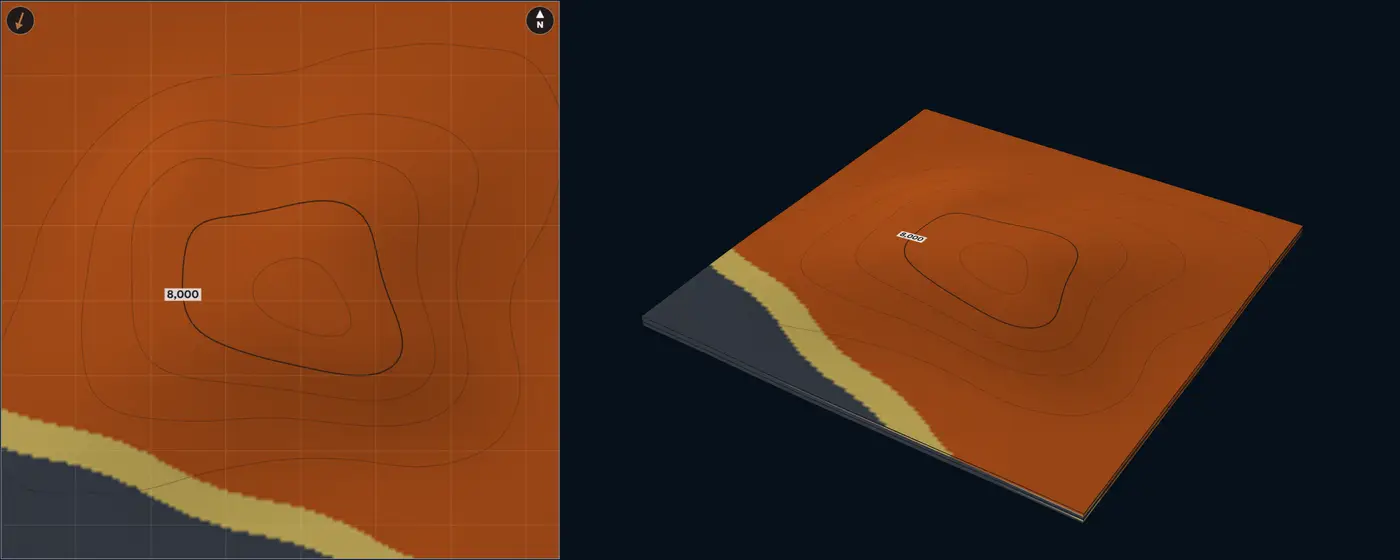
- Foreshore and upper shoreface
- Lower shoreface
- Offshore transition
- Swale mud
- Mudstone and shale
| Size | Default | Published | From |
|---|---|---|---|
| Shoreface sand-body width | 8.08 mi13 km | 4.35 to 15.5 mi7 to 25 km | Reynolds (1999) |
| Shoreface clinoform length | 7,220 ft2,200 m | 2,625 to 19,685 ft800 to 6,000 m | Hampson (2000) |
| Parasequence thickness | 49 ft15 m | Lab setting, no compiled range | – |
| Beach-ridge spacing | 1,310 ft400 m | Lab setting, no compiled range | – |
| Shoreline spread | 5° | Lab setting, no compiled range | – |
Sources for this architecture
Reynolds (1999)
Reynolds, A. D., 1999, Dimensions of paralic sandstone bodies: AAPG Bulletin, v. 83, no. 2, p. 211–229. doi:10.1306/00AA9A48-1730-11D7-8645000102C1865D (opens in a new tab)
Hampson (2000)
Hampson, G. J., 2000, Discontinuity Surfaces, Clinoforms, and Facies Architecture in a Wave-Dominated, Shoreface-Shelf Parasequence: Journal of Sedimentary Research, v. 70, no. 2, p. 325–340. doi:10.1306/2DC40914-0E47-11D7-8643000102C1865D (opens in a new tab)
Hampson and Storms (2003)
Hampson, G. J., and Storms, J. E. A., 2003, Geomorphological and sequence stratigraphic variability in wave-dominated, shoreface-shelf parasequences: Sedimentology, v. 50, no. 4, p. 667–701. doi:10.1046/j.1365-3091.2003.00570.x (opens in a new tab)
Clifton (2006)
Clifton, H. E., 2006, A Reexamination of Facies Models for Clastic Shorelines: in Facies Models Revisited: SEPM Special Publication 84, p. 293–337. doi:10.2110/pec.06.84.0293 (opens in a new tab)
Bhattacharya and Giosan (2003)
Bhattacharya, J. P., and Giosan, L., 2003, Wave-influenced deltas: geomorphological implications for facies reconstruction: Sedimentology, v. 50, no. 1, p. 187–210. doi:10.1046/j.1365-3091.2003.00545.x (opens in a new tab)
Tide-dominated delta with tidal bars Shallow marine Elongate tidal bars in a funnel-shaped mouth
Geometry
Tidal currents shape the mouth into a seaward-widening funnel and its sand into elongate bars parallel to the flow. On coasts with tidal ranges over 9.8 ft3 m, tidal current ridges are 26 to 98 ft8 to 30 m high, 4.97 to 39.8 mi8 to 64 km long and 0.99 to 6.03 mi1.6 to 9.7 km apart, their spacing proportional to water depth (Off 1963, converted from feet and miles); the lab uses those ranges for the bars. On the Fly River delta three main distributaries flare seaward from a bifurcation 68.4 mi110 km inland, with elongate tidal bars in the distributaries and the mouth-bar area (Dalrymple et al. 2003).
Facies
Tidal bars of cross-bedded sand with mud drapes, their heterolithic margins, tidal flats and channel floors, prodelta mud. On the Fly the bars may hold 50% mud or more and show lateral-accretion bedding; channel floors are thin sand under fluid-mud deposits (Dalrymple et al. 2003). In the Cobequid Bay estuary, the seaward tidal bars build out into a 66 ft20 m thick fining-up succession whose lower half to two-thirds is cross-bedded medium to coarse sand (Dalrymple et al. 1990). The lab counts the bar core 80% net, its margin 50% and the flats 28%.
NTG behaviour
Linear: wells along one bar agree, and wells across the bars alternate between bar sand and heterolithic flats about one bar spacing apart. NTG drops to prodelta mud beyond the delta front.
Modern analogue
Fly River delta, Papua New Guinea. Spring tides up to 16 ft5 m and near-bed currents over 1 m/s; after the postglacial sea-level rise its mouth bars built out by as much as 24.9 to 31.1 mi40 to 50 km (Dalrymple et al. 2003). Mitchell River delta, Gulf of Carpentaria. A modern tide-dominated delta of more than 193 mi²500 km², whose wave-formed sand bodies are much longer for their width than its fluvial ones (Nanson et al. 2012).
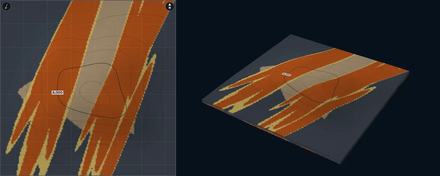
- Tidal bar
- Tidal-bar margin, heterolithic
- Tidal flat and channel heterolithics
- Mudstone and shale
| Size | Default | Published | From |
|---|---|---|---|
| Tidal-bar length | 12.4 mi20 km | 4.97 to 39.8 mi8 to 64 km | Off (1963) |
| Tidal-bar height | 49 ft15 m | 26 to 98 ft8 to 30 m | Off (1963) |
| Tidal-bar spacing | 2.49 mi4 km | 0.99 to 6.03 mi1.6 to 9.7 km | Off (1963) |
| Tidal-bar width | 0.75 mi1.2 km | Lab setting, no compiled range | – |
| Paleoflow spread | 8° | Lab setting, no compiled range | – |
Sources for this architecture
Off (1963)
Off, T., 1963, Rhythmic Linear Sand Bodies Caused by Tidal Currents: AAPG Bulletin, v. 47, no. 2, p. 324–341. doi:10.1306/BC743989-16BE-11D7-8645000102C1865D (opens in a new tab)
Dalrymple et al. (2003)
Dalrymple, R. W., Baker, E. K., Harris, P. T., and Hughes, M. G., 2003, Sedimentology and Stratigraphy of a Tide-Dominated, Foreland-Basin Delta (Fly River, Papua New Guinea): in Tropical Deltas of Southeast Asia: Sedimentology, Stratigraphy, and Petroleum Geology: SEPM Special Publication 76, p. 147–173. doi:10.2110/pec.03.76.0147 (opens in a new tab)
Dalrymple et al. (1990)
Dalrymple, R. W., Knight, R. J., Zaitlin, B. A., and Middleton, G. V., 1990, Dynamics and facies model of a macrotidal sand-bar complex, Cobequid Bay—Salmon River Estuary (Bay of Fundy): Sedimentology, v. 37, no. 4, p. 577–612. doi:10.1111/j.1365-3091.1990.tb00624.x (opens in a new tab)
Nanson et al. (2012)
Nanson, R., Ainsworth, B., Vakarelov, B., Fernie, A., and Massey, T., 2012, Geometric attributes of reservoir elements in a modern, low accomodation, tide-dominated delta: The APPEA Journal, v. 52, no. 1, p. 483–492. doi:10.1071/AJ11038 (opens in a new tab)
Incised-valley fill Estuarine A lowstand valley filled with fluvial and estuarine deposits
Geometry
A valley cut during a fall in relative sea level and filled mostly during the following rise. Valleys average about 6.21 mi10 km wide, with aspect ratios of the order of 1:1,000, much wider than channels (Reynolds 1999). Across 151 late-Quaternary valley fills, those on active margins are thicker and wider than those on passive margins, and fill size grows with the drainage basin (Wang et al. 2019). A simple fill records one cycle of incision and filling, a compound fill several (Zaitlin et al. 1994).
Facies
Lowstand fluvial sand on the thalweg, then estuarine sand and bayhead deltas, central-basin estuarine mud and transgressive marine sand, each unit onlapping the valley walls. Estuaries have a marine sand body at the mouth, a muddy central basin and a bayhead delta (Dalrymple et al. 1992). In the Gironde, lowstand gravel and coarse sand floor the thalweg and tidal-estuarine sands and muds make most of the fill (Allen and Posamentier 1993). Fills on active margins hold more fluvial and less central-basin deposit than those on passive margins (Wang et al. 2020). The lab counts the fluvial sand 90% net, estuarine sand 65%, central-basin mud 8% and transgressive sand 45%.
NTG behaviour
Sand stays inside the valley, best at its base along the thalweg and thinning onto the walls; the interfluves are mud. Two wells in one valley differ when one sits on the thalweg and the other on a wall.
Modern analogue
Gironde Estuary, France. A fluvial valley cut during the last glacial lowstand, drowned in the Holocene and now filling with a tide-dominated bayhead delta (Allen and Posamentier 1993).
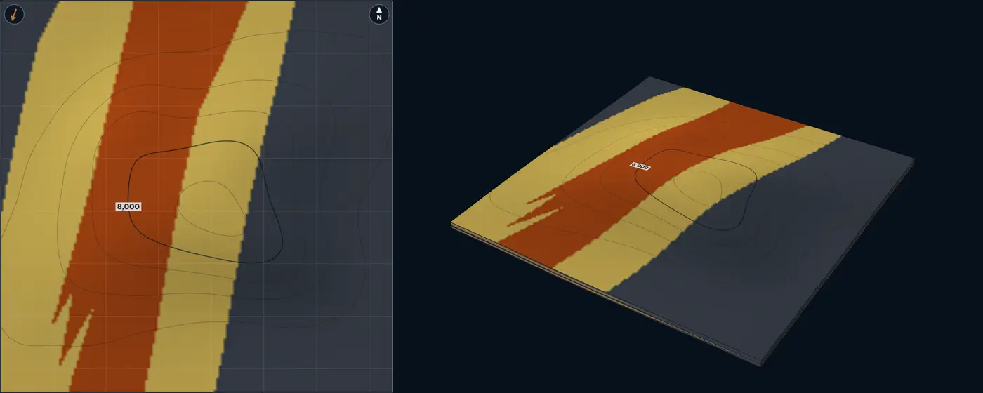
- Lowstand fluvial sand
- Estuarine sand and bayhead delta
- Transgressive marine sand
- Central-basin estuarine mud
- Mudstone and shale
| Size | Default | Published | From |
|---|---|---|---|
| Valley width | 6.21 mi10 km | Average about 6.21 mi10 km | Reynolds (1999) |
| Valley-fill thickness | 33 ft10 m | Lab setting, no compiled range | – |
| Lowstand fluvial share | 0.3 | Lab setting, no compiled range | – |
| Paleoflow spread | 8° | Lab setting, no compiled range | – |
| Width / thickness | 1,000 | Of the order of 1,000 | Reynolds (1999) |
Sources for this architecture
Reynolds (1999)
Reynolds, A. D., 1999, Dimensions of paralic sandstone bodies: AAPG Bulletin, v. 83, no. 2, p. 211–229. doi:10.1306/00AA9A48-1730-11D7-8645000102C1865D (opens in a new tab)
Wang et al. (2019)
Wang, R., Colombera, L., and Mountney, N. P., 2019, Geological controls on the geometry of incised-valley fills: Insights from a global dataset of late-Quaternary examples: Sedimentology, v. 66, no. 6, p. 2134–2168. doi:10.1111/sed.12596 (opens in a new tab)
Zaitlin et al. (1994)
Zaitlin, B. A., Dalrymple, R. W., and Boyd, R., 1994, The Stratigraphic Organization of Incised-Valley Systems Associated with Relative Sea-Level Change: in Incised-Valley Systems: Origin and Sedimentary Sequences: SEPM Special Publication 51, p. 45–60. doi:10.2110/pec.94.12.0045 (opens in a new tab)
Dalrymple et al. (1992)
Dalrymple, R. W., Zaitlin, B. A., and Boyd, R., 1992, Estuarine facies models; conceptual basis and stratigraphic implications: Journal of Sedimentary Research, v. 62, no. 6, p. 1130–1146. doi:10.1306/D4267A69-2B26-11D7-8648000102C1865D (opens in a new tab)
Allen and Posamentier (1993)
Allen, G. P., and Posamentier, H. W., 1993, Sequence stratigraphy and facies model of an incised valley fill; the Gironde Estuary, France: Journal of Sedimentary Research, v. 63, no. 3, p. 378–391. doi:10.1306/D4267B09-2B26-11D7-8648000102C1865D (opens in a new tab)
Wang et al. (2020)
Wang, R., Colombera, L., and Mountney, N. P., 2020, Quantitative analysis of the stratigraphic architecture of incised-valley fills: A global comparison of Quaternary systems: Earth-Science Reviews, v. 200, p. 102988. doi:10.1016/j.earscirev.2019.102988 (opens in a new tab)
Shelf to shelf-slope break
Shelf-edge delta Shelf margin A delta at the shelf edge, feeding the slope
Geometry
The delta front sits at the shelf-slope break, where the clinoform steepens onto the upper slope, and gullies carry its sand downslope. Across some 29 shelf-margin clinoforms, river-dominated shelf-edge deltas are a reliable sign that sand reached deep water (Dixon et al. 2012). Shelf-margin clinoforms in front of shelves 6.21 to 37.3 mi10 to 60 km wide have slopes of 2 to 4 degrees, and river-dominated deltas put sand beyond the shelf-slope break most efficiently (Johannessen and Steel 2005). Delta-scale clinoforms are the smallest kind (Patruno et al. 2015).
Facies
Distributary channels and mouth bars on the outer shelf, a proximal and distal delta front over the shelf edge, gully fills on the upper slope, slope mud. Shelf-margin deltas link shelf sands with deepwater sands (Porębski and Steel 2003). The lab counts distributary fill 90% net, mouth bars 84%, gully fill 60%, the proximal front 48% and the distal front 28%.
NTG behaviour
Sand gathers at the shelf edge in front of the river mouth and runs down the slope only in the gullies, so an upper-slope well reads high in a gully and near zero between gullies.
Analogue
Offshore Trinidad, near the Orinoco Delta. Plio-Pleistocene shelf-edge deltas fed shelf-attached mass-transport complexes (Moscardelli and Wood 2008). Eocene Central Basin, Spitsbergen. Outcropping shelf-margin clinoforms, where flat, channelled shelf-edge trajectories go with deepwater sands (Johannessen and Steel 2005).
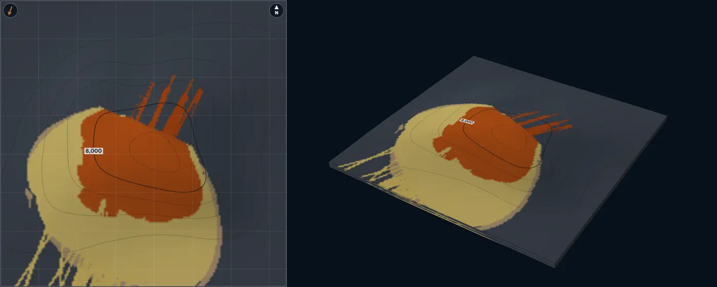
- Distributary channel
- Mouth-bar core
- Proximal delta front
- Upper-slope gully fill
- Distal delta front and prodelta
- Mudstone and shale
| Size | Default | Published | From |
|---|---|---|---|
| Delta-front height | 98 ft30 m | 3.3 to 195 ft1 to 60 m | Patruno et al. (2015) |
| Upper-slope gradient | 3° | 2 to 4° | Johannessen and Steel (2005) |
| Mouth-bar length | 1.86 mi3 km | 0.62 to 6.21 mi1 to 10 km | Ainsworth et al. (2016); Reynolds (1999) |
| Gully width | 655 ft200 m | Lab setting, no compiled range | – |
| Delta-lobe length | 3.11 mi5 km | Lab setting, no compiled range | – |
| Paleoflow spread | 12° | Lab setting, no compiled range | – |
Sources for this architecture
Dixon et al. (2012)
Dixon, J. F., Steel, R. J., and Olariu, C., 2012, Shelf-Edge Delta Regime As A Predictor of Deep-Water Deposition: Journal of Sedimentary Research, v. 82, no. 9, p. 681–687. doi:10.2110/jsr.2012.59 (opens in a new tab)
Johannessen and Steel (2005)
Johannessen, E. P., and Steel, R. J., 2005, Shelf-margin clinoforms and prediction of deepwater sands: Basin Research, v. 17, no. 4, p. 521–550. doi:10.1111/j.1365-2117.2005.00278.x (opens in a new tab)
Patruno et al. (2015)
Patruno, S., Hampson, G. J., and Jackson, C. A.-L., 2015, Quantitative characterisation of deltaic and subaqueous clinoforms: Earth-Science Reviews, v. 142, p. 79–119. doi:10.1016/j.earscirev.2015.01.004 (opens in a new tab)
Porębski and Steel (2003)
Porębski, S. J., and Steel, R. J., 2003, Shelf-margin deltas: their stratigraphic significance and relation to deepwater sands: Earth-Science Reviews, v. 62, no. 3–4, p. 283–326. doi:10.1016/S0012-8252(02)00161-7 (opens in a new tab)
Moscardelli and Wood (2008)
Moscardelli, L., and Wood, L., 2008, New classification system for mass transport complexes in offshore Trinidad: Basin Research, v. 20, no. 1, p. 73–98. doi:10.1111/j.1365-2117.2007.00340.x (opens in a new tab)
Ainsworth et al. (2016)
Ainsworth, R. B., Vakarelov, B. K., MacEachern, J. A., Nanson, R. A., Lane, T. I., Rarity, F., and Dashtgard, S. E., 2016, Process-driven architectural variability in mouth-bar deposits: a case study from a mixed-process mouth-bar complex, Drumheller, Alberta, Canada: Journal of Sedimentary Research, v. 86, no. 5, p. 512–541. doi:10.2110/jsr.2016.23 (opens in a new tab)
Reynolds (1999)
Reynolds, A. D., 1999, Dimensions of paralic sandstone bodies: AAPG Bulletin, v. 83, no. 2, p. 211–229. doi:10.1306/00AA9A48-1730-11D7-8645000102C1865D (opens in a new tab)
Shelf-margin clinoforms Shelf margin Topset, foreset and bottomset belts
Geometry
The shelf edge crosses the block: the topset lies landward, the foreset down the slope and the bottomset at its toe. Shelf-edge clinoforms are hundreds of metres high and build out over 0.1 to 20 million years at 3.3 to 330 ft1 to 100 m per thousand years, through repeated crossings of the shelf by delta-scale clinoforms (Patruno and Helland-Hansen 2018). The lab builds the shelf edge out within the zone by the zone’s thickness over the tangent of the trajectory angle, so the facies belts step basinward as they climb.
Facies
Topset sandstone, a sand-prone upper foreset, a muddier lower foreset and bottomset, and toe-of-slope turbidites where sand bypasses the slope. Flat, channelled shelf-edge trajectories go with sandy slopes and basin floors, rising ones with muddy slopes (Johannessen and Steel 2005); descending trajectories bring few, thin shoreline tongues and high sediment supply to basin-floor fans (Helland-Hansen and Hampson 2009). The lab counts the topset 80% net, upper foreset 45%, lower foreset and bottomset 18% and toe-of-slope turbidites 62%.
NTG behaviour
Belts parallel to the shelf edge: high on the topset, falling down the foreset, rising again at the toe only where turbidites reached it. Every column coarsens up as the margin builds out over it.
Analogue
Eocene, Spitsbergen and offshore Ireland. Shelf-margin clinoforms in outcrop and in seismic, with slopes of 2 to 4 degrees in front of shelves 6.21 to 37.3 mi10 to 60 km wide (Johannessen and Steel 2005).
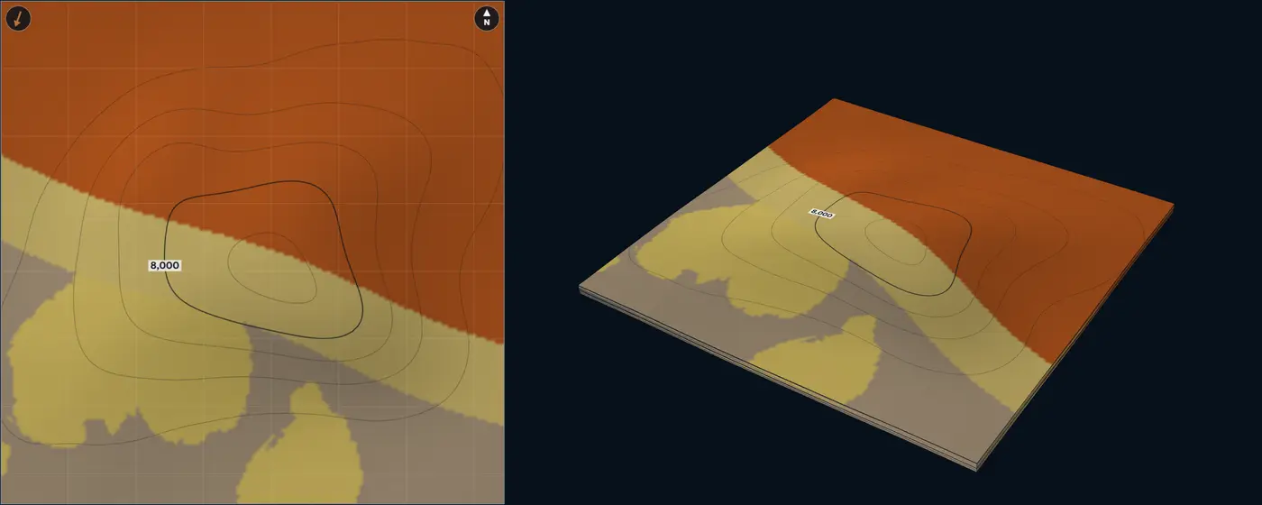
- Topset sandstone
- Upper foreset
- Toe-of-slope turbidites
- Lower foreset and bottomset
- Mudstone and shale
| Size | Default | Published | From |
|---|---|---|---|
| Clinoform height | 985 ft300 m | 330 to 2,955 ft100 to 900 m | Patruno and Helland-Hansen (2018) |
| Foreset gradient | 3° | 2 to 4° | Johannessen and Steel (2005) |
| Shelf-edge trajectory | 0.5° | Lab setting, no compiled range | – |
| Shelf-edge spread | 5° | Lab setting, no compiled range | – |
Sources for this architecture
Patruno and Helland-Hansen (2018)
Patruno, S., and Helland-Hansen, W., 2018, Clinoforms and clinoform systems: Review and dynamic classification scheme for shorelines, subaqueous deltas, shelf edges and continental margins: Earth-Science Reviews, v. 185, p. 202–233. doi:10.1016/j.earscirev.2018.05.016 (opens in a new tab)
Johannessen and Steel (2005)
Johannessen, E. P., and Steel, R. J., 2005, Shelf-margin clinoforms and prediction of deepwater sands: Basin Research, v. 17, no. 4, p. 521–550. doi:10.1111/j.1365-2117.2005.00278.x (opens in a new tab)
Helland-Hansen and Hampson (2009)
Helland-Hansen, W., and Hampson, G. J., 2009, Trajectory analysis: concepts and applications: Basin Research, v. 21, no. 5, p. 454–483. doi:10.1111/j.1365-2117.2009.00425.x (opens in a new tab)
Patruno et al. (2015)
Patruno, S., Hampson, G. J., and Jackson, C. A.-L., 2015, Quantitative characterisation of deltaic and subaqueous clinoforms: Earth-Science Reviews, v. 142, p. 79–119. doi:10.1016/j.earscirev.2015.01.004 (opens in a new tab)
Slope
Confined slope channel complex Slope Slope channel complex in a confining belt
Geometry
Channel elements, each a single channel fill, stack inside a belt cut into the slope. Submarine channel belts build mostly upward: about 9 times wider than thick, against about 72 for river belts (Jobe et al. 2016). In the schemes Cullis et al. (2018) compare, single-storey channels are up to 23 ft7 m thick and 655 ft200 m wide, channel-fill elements average 46 ft14 m thick and 3,280 ft1,000 m wide, and channel complexes average 120 ft37 m thick and 4,595 ft1,400 m wide. Modern channels are 10 to 100 times wider than deep (Shumaker et al. 2018).
Sinuosity on the Amazon Channel stays below 1.5 where the valley slope is steeper than 8 m/km and reaches about 2.3, varying from 1.2 to 2.7, farther down the fan (Pirmez and Flood 1995). High-latitude channels peak near 1.4 (Allen et al. 2022). The lab defaults to 1.3, a slope channel.
Facies
Each fill grades from a sandy axis to a muddier margin, with thin-bedded internal levees beside it, all inside the belt; outside it is mud. The lab counts the axis 93% net, the margin 62% and the levees 28%.
NTG behaviour
Sand is linear. A well in the belt axis can read 80% with mud a belt-width away, wells strung along the belt agree, and wells across it do not. Belt width and the number of belts cap how much of the block can be sand.
Modern analogue
Congo (Zaire) Channel, offshore West Africa. A meandering channel whose thalweg is cut well below the regional sea floor along its whole length, which limits overflow onto the levees and prevents avulsion along its upper part (Babonneau et al. 2002). Amazon Channel. 0.5 to 0.81 mi0.8 to 1.3 km wide on the middle fan, with width-to-relief ratios of 10 to 40 (Pirmez and Flood 1995).
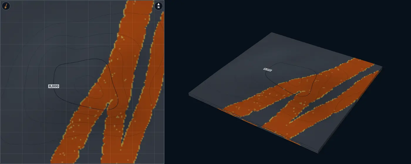
- Channel axis
- Channel margin
- Levee and overbank
- Mudstone and shale
| Size | Default | Published | From |
|---|---|---|---|
| Channel width | 1,150 ft350 m | 330 to 3,280 ft100 to 1,000 m | Cullis et al. (2018); Cullis et al. (2019); Shumaker et al. (2018) |
| Channel thickness | 33 ft10 m | 3.3 to 98 ft1 to 30 m | Cullis et al. (2018) |
| Sinuosity | 1.3 | 1 to 2.7 | Pirmez and Flood (1995); Allen et al. (2022) |
| Belt width | 4,595 ft1,400 m | 3,280 to 9,845 ft1,000 to 3,000 m | Cullis et al. (2018); Jobe et al. (2016) |
| Paleoflow spread | 10° | Lab setting, no compiled range | – |
| Width / thickness | 35 | 10 to 100 | Shumaker et al. (2018); Clark and Pickering (1996); Konsoer et al. (2013); Cullis et al. (2019) |
Sources for this architecture
Jobe et al. (2016)
Jobe, Z. R., Howes, N. C., and Auchter, N. C., 2016, Comparing submarine and fluvial channel kinematics: implications for stratigraphic architecture: Geology, v. 44, no. 11, p. 931–934. doi:10.1130/G38158.1 (opens in a new tab)
Cullis et al. (2018)
Cullis, S., Colombera, L., Patacci, M., and McCaffrey, W. D., 2018, Hierarchical classifications of the sedimentary architecture of deep-marine depositional systems: Earth-Science Reviews, v. 179, p. 38–71. doi:10.1016/j.earscirev.2018.01.016 (opens in a new tab)
Cullis et al. (2019)
Cullis, S., Patacci, M., Colombera, L., Bührig, L., and McCaffrey, W. D., 2019, A database solution for the quantitative characterisation and comparison of deep-marine siliciclastic depositional systems: Marine and Petroleum Geology, v. 102, p. 321–339. doi:10.1016/j.marpetgeo.2018.12.023 (opens in a new tab)
Shumaker et al. (2018)
Shumaker, L. E., Jobe, Z. R., Johnstone, S. A., Pettinga, L. A., Cai, D., and Moody, J. D., 2018, Controls on submarine channel-modifying processes identified through morphometric scaling relationships: Geosphere, v. 14, no. 5, p. 2171–2187. doi:10.1130/GES01674.1 (opens in a new tab)
Clark and Pickering (1996)
Clark, J. D., and Pickering, K. T., 1996, Architectural elements and growth patterns of submarine channels: application to hydrocarbon exploration: AAPG Bulletin, v. 80, no. 2, p. 194–220. doi:10.1306/64ED878C-1724-11D7-8645000102C1865D (opens in a new tab)
Konsoer et al. (2013)
Konsoer, K., Zinger, J., and Parker, G., 2013, Bankfull hydraulic geometry of submarine channels created by turbidity currents: relations between bankfull channel characteristics and formative flow discharge: Journal of Geophysical Research: Earth Surface, v. 118, no. 1, p. 216–228. doi:10.1029/2012JF002422 (opens in a new tab)
Pirmez and Flood (1995)
Pirmez, C., and Flood, R. D., 1995, Morphology and structure of Amazon Channel: Proceedings of the Ocean Drilling Program, Initial Reports, v. 155. doi:10.2973/odp.proc.ir.155.103.1995 (opens in a new tab)
Allen et al. (2022)
Allen, C., Peakall, J., Hodgson, D. M., Bradbury, W., and Booth, A. D., 2022, Latitudinal changes in submarine channel-levee system evolution, architecture and flow processes: Frontiers in Earth Science, v. 10, article 976852. doi:10.3389/feart.2022.976852 (opens in a new tab)
Babonneau et al. (2002)
Babonneau, N., Savoye, B., Cremer, M., and Klein, B., 2002, Morphology and architecture of the present canyon and channel system of the Zaire deep-sea fan: Marine and Petroleum Geology, v. 19, no. 4, p. 445–467. doi:10.1016/S0264-8172(02)00009-0 (opens in a new tab)
Leveed channel with overbank Slope A sinuous channel between thinning external levees
Geometry
Turbidity-flow leveed channels range from less than 655 ft200 m to more than 1.86 mi3 km wide, with moderate to high sinuosity, and their meanders mostly migrate down-system (Posamentier and Kolla 2003). Across six channel-levee systems, levee thickness falls exponentially away from the channel, and the levee’s e-folding width and length scale with channel width and relief (Skene et al. 2002). On slopes steeper than about 0.6 degrees the decay follows a power law instead, and gentle basin floors carry wider levees (Nakajima and Kneller 2013). The lab uses the exponential form.
Facies
Channel axis and margin fills, levees of thin-bedded turbidites thinning and fining away from the channel, overbank splays where flows breach the levee at bends, mud beyond. High-sinuosity channels can build overbank sediment waves up to 66 ft20 m high and 1.24 to 1.86 mi2 to 3 km apart, and crevasse splays form where levees are breached, commonly at bends (Posamentier and Kolla 2003). The lab counts the axis 93% net, margin 62%, splays 55% and levees 28%.
NTG behaviour
Sandy along the channel; the levees add thin-bedded sand that thins away from it over kilometres, so NTG falls gradually across the overbank, not in a step.
Modern analogue
Amazon Channel. A leveed channel on the Amazon Fan, 0.5 to 0.81 mi0.8 to 1.3 km wide on the middle fan with width-to-relief ratios of 10 to 40 (Pirmez and Flood 1995).
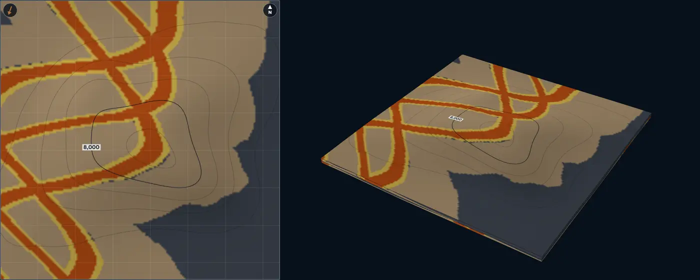
- Channel axis
- Channel margin
- Overbank splay
- Levee and overbank
- Mudstone and shale
| Size | Default | Published | From |
|---|---|---|---|
| Channel width | 4,265 ft1,300 m | 655 to 9,845 ft200 to 3,000 m | Posamentier and Kolla (2003) |
| Channel relief | 195 ft60 m | Lab setting, no compiled range | – |
| Sinuosity | 1.3 | 1 to 2.7 | Pirmez and Flood (1995) |
| Levee e-folding width | 1.55 mi2.5 km | Lab setting, no compiled range | – |
| Overbank-splay length | 1.86 mi3 km | Lab setting, no compiled range | – |
| Paleoflow spread | 10° | Lab setting, no compiled range | – |
| Width / relief | 21.7 | 10 to 40 | Pirmez and Flood (1995) |
Sources for this architecture
Posamentier and Kolla (2003)
Posamentier, H. W., and Kolla, V., 2003, Seismic Geomorphology and Stratigraphy of Depositional Elements in Deep-Water Settings: Journal of Sedimentary Research, v. 73, no. 3, p. 367–388. doi:10.1306/111302730367 (opens in a new tab)
Skene et al. (2002)
Skene, K. I., Piper, D. J. W., and Hill, P. S., 2002, Quantitative analysis of variations in depositional sequence thickness from submarine channel levees: Sedimentology, v. 49, no. 6, p. 1411–1430. doi:10.1046/j.1365-3091.2002.00506.x (opens in a new tab)
Nakajima and Kneller (2013)
Nakajima, T., and Kneller, B. C., 2013, Quantitative analysis of the geometry of submarine external levées: Sedimentology, v. 60, no. 4, p. 877–910. doi:10.1111/j.1365-3091.2012.01366.x (opens in a new tab)
Pirmez and Flood (1995)
Pirmez, C., and Flood, R. D., 1995, Morphology and structure of Amazon Channel: Proceedings of the Ocean Drilling Program, Initial Reports, v. 155. doi:10.2973/odp.proc.ir.155.103.1995 (opens in a new tab)
Slope MTD with ponded sands Slope A mass-transport deposit whose rugose top ponds sand
Geometry
A mass-transport deposit spreads over the slope with steep edges and a rugose top. Offshore Trinidad, mass-transport complexes cover 4.36 to 779 mi²11.3 to 2,017 km² (Moscardelli and Wood 2008); the largest deposits cover more than 3,861 mi²10,000 km² and are more than 330 ft100 m thick (Kneller et al. 2016), and single debris-flow units reach 260 ft80 m (Posamentier and Kolla 2003). At Sierra Contreras, Chile, relief on deposit tops comes in three tiers, each about ten times the last: up to several metres, then tens of metres, then several hundred metres across (Armitage et al. 2009).
Facies
The mass-transport deposit (a mud-rich debrite), ponded turbidite sandstone in the lows of its top, healing-phase turbidites that drape and smooth the relief, thin-bedded turbidites lapping onto its highs, slope mud. Sandstone beds pinch out and lap onto the highs of the deposit’s top, and as the relief heals the turbidites become more laterally continuous (Armitage et al. 2009). Debris-flow deposits are mud-rich (Posamentier and Kolla 2003). The lab counts ponded sand 88% net, healing-phase turbidites 62%, thin beds 32% and the deposit itself 8%.
NTG behaviour
Low and patchy: sand sits in pockets a few hundred metres across, compartmentalized by the deposit’s relief, and becomes more continuous upward. Wells a kilometre apart rarely share a pocket.
Analogue
Sierra Contreras, southern Chile. Tres Pasos Formation outcrops where turbidites pond on, then heal, the tops of mass-transport deposits (Armitage et al. 2009). Offshore Trinidad. Plio-Pleistocene mass-transport complexes mapped on 4,134 mi²10,708 km² of 3D seismic (Moscardelli and Wood 2008).
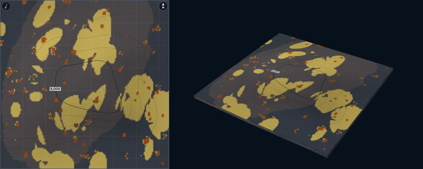
- Ponded turbidite sandstone
- Healing-phase turbidites
- Thin-bedded turbidites
- Mass-transport deposit
- Mudstone and shale
| Size | Default | Published | From |
|---|---|---|---|
| MTD area | 58 mi²150 km² | 4.36 to 779 mi²11.3 to 2,017 km² | Moscardelli and Wood (2008) |
| MTD thickness | 82 ft25 m | up to 260 ft80 m | Posamentier and Kolla (2003) |
| Ponded-sand pocket width | 1,310 ft400 m | 655 to 2,955 ft200 to 900 m | Armitage et al. (2009) |
| Ponded-sand thickness | 26 ft8 m | Lab setting, no compiled range | – |
| Paleoflow spread | 10° | Lab setting, no compiled range | – |
Sources for this architecture
Moscardelli and Wood (2008)
Moscardelli, L., and Wood, L., 2008, New classification system for mass transport complexes in offshore Trinidad: Basin Research, v. 20, no. 1, p. 73–98. doi:10.1111/j.1365-2117.2007.00340.x (opens in a new tab)
Kneller et al. (2016)
Kneller, B., Dykstra, M., Fairweather, L., and Milana, J. P., 2016, Mass-transport and slope accommodation: Implications for turbidite sandstone reservoirs: AAPG Bulletin, v. 100, no. 2, p. 213–235. doi:10.1306/09011514210 (opens in a new tab)
Posamentier and Kolla (2003)
Posamentier, H. W., and Kolla, V., 2003, Seismic Geomorphology and Stratigraphy of Depositional Elements in Deep-Water Settings: Journal of Sedimentary Research, v. 73, no. 3, p. 367–388. doi:10.1306/111302730367 (opens in a new tab)
Armitage et al. (2009)
Armitage, D. A., Romans, B. W., Covault, J. A., and Graham, S. A., 2009, The Influence of Mass-Transport-Deposit Surface Topography on the Evolution of Turbidite Architecture: The Sierra Contreras, Tres Pasos Formation (Cretaceous), Southern Chile: Journal of Sedimentary Research, v. 79, no. 5, p. 287–301. doi:10.2110/jsr.2009.035 (opens in a new tab)
Basin floor and deepwater
Distributary lobe channel Deepwater A lobe built at the mouth of its feeder channel
Geometry
Lobes in the late Pleistocene fans off East Corsica cover 1.16 to 27 mi²3 to 70 km², run 1.24 to more than 8.7 mi2 to more than 14 km down-flow and 0.62 to more than 6.21 mi1 to more than 10 km across, with length-to-width ratios of 1 to 3, peak thicknesses of 26 to 140 ft8 to 42 m and thickness-to-width ratios of 0.001 to 0.0065 (Deptuck et al. 2008). In outcrop, lobes are commonly 9.8 to 49 ft3 to 15 m thick (Mutti and Normark, as cited by Deptuck et al. 2008). Lobe elements step 1,640 to 6,560 ft500 to 2,000 m aside from one another as they build a composite lobe (Deptuck et al. 2008, as summarised by Cullis et al. 2018); the lab uses that step here.
Facies
Lobe axis, off-axis and fringe in arcs around the feeder mouth, with the feeder and its short distributaries cutting the proximal lobe. In the Karoo, thin-bedded siltstones separate successive lobes, and lobe fringes can thin abruptly into fingers without erosion (Prélat et al. 2009). The lab counts the lobe axis 88% net, off-axis 66% and fringe 35%.
NTG behaviour
Sand concentrates along the feeder and near the channel mouth and fades to the fringe within a few kilometres. On the modern Congo lobe complex sand is about 13% of the deposit and lies in the feeding channel and distributaries; the lobe body is thin, muddy to silty turbidites (Dennielou et al. 2017).
Modern analogue
Congo channel-mouth lobe complex, Angola abyssal plain. Active today, 55.9 by 24.9 mi90 by 40 km (975 mi²2,525 km²), 472 mi760 km from the river mouth, built of five lobes that have prograded (Dennielou et al. 2017).
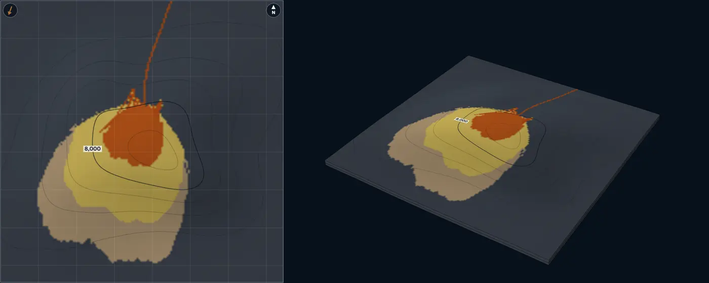
- Channel axis
- Lobe axis
- Channel margin
- Lobe off-axis
- Lobe fringe
- Levee and overbank
- Mudstone and shale
| Size | Default | Published | From |
|---|---|---|---|
| Lobe length | 3.73 mi6 km | 1.24 to 8.7 mi2 to 14 km | Deptuck et al. (2008) |
| Lobe width | 1.86 mi3 km | 0.62 to 6.21 mi1 to 10 km | Deptuck et al. (2008) |
| Lobe thickness | 26 ft8 m | 9.8 to 140 ft3 to 42 m | Deptuck et al. (2008); Prélat, Hodgson and Flint (2009) |
| Feeder channel width | 820 ft250 m | 330 to 3,280 ft100 to 1,000 m | Cullis et al. (2018); Cullis et al. (2019) |
| Feeder channel thickness | 20 ft6 m | 3.3 to 98 ft1 to 30 m | Cullis et al. (2018) |
| Compensation offset | 0.62 mi1 km | 0.31 to 1.24 mi0.5 to 2 km | Deptuck et al. (2008); Cullis et al. (2018) |
| Paleoflow spread | 10° | Lab setting, no compiled range | – |
| Length / width | 2 | 1 to 3 | Deptuck et al. (2008) |
| Lobe width / thickness | 375 | 150 to 1,000 | Deptuck et al. (2008) |
| Feeder width / thickness | 41.7 | 10 to 100 | Shumaker et al. (2018); Cullis et al. (2019) |
Sources for this architecture
Deptuck et al. (2008)
Deptuck, M. E., Piper, D. J. W., Savoye, B., and Gervais, A., 2008, Dimensions and architecture of late Pleistocene submarine lobes off the northern margin of East Corsica: Sedimentology, v. 55, no. 4, p. 869–898. doi:10.1111/j.1365-3091.2007.00926.x (opens in a new tab)
Cullis et al. (2018)
Cullis, S., Colombera, L., Patacci, M., and McCaffrey, W. D., 2018, Hierarchical classifications of the sedimentary architecture of deep-marine depositional systems: Earth-Science Reviews, v. 179, p. 38–71. doi:10.1016/j.earscirev.2018.01.016 (opens in a new tab)
Prélat, Hodgson and Flint (2009)
Prélat, A., Hodgson, D. M., and Flint, S. S., 2009, Evolution, architecture and hierarchy of distributary deep-water deposits: a high-resolution outcrop investigation from the Permian Karoo Basin, South Africa: Sedimentology, v. 56, no. 7, p. 2132–2154. doi:10.1111/j.1365-3091.2009.01073.x (opens in a new tab)
Dennielou et al. (2017)
Dennielou, B., Droz, L., Babonneau, N., Jacq, C., Bonnel, C., Picot, M., Le Saout, M., Saout, Y., Bez, M., Savoye, B., Olu, K., and Rabouille, C., 2017, Morphology, structure, composition and build-up processes of the active channel-mouth lobe complex of the Congo deep-sea fan with inputs from remotely operated underwater vehicle (ROV) multibeam and video surveys: Deep-Sea Research Part II, v. 142, p. 25–49. doi:10.1016/j.dsr2.2017.03.010 (opens in a new tab)
Cullis et al. (2019)
Cullis, S., Patacci, M., Colombera, L., Bührig, L., and McCaffrey, W. D., 2019, A database solution for the quantitative characterisation and comparison of deep-marine siliciclastic depositional systems: Marine and Petroleum Geology, v. 102, p. 321–339. doi:10.1016/j.marpetgeo.2018.12.023 (opens in a new tab)
Shumaker et al. (2018)
Shumaker, L. E., Jobe, Z. R., Johnstone, S. A., Pettinga, L. A., Cai, D., and Moody, J. D., 2018, Controls on submarine channel-modifying processes identified through morphometric scaling relationships: Geosphere, v. 14, no. 5, p. 2171–2187. doi:10.1130/GES01674.1 (opens in a new tab)
Lobe-channel complex Deepwater Several lobes, each filling the low beside the last
Geometry
Lobes, each with its own feeder, stack where the previous lobes left a low. The thickest parts of successive composite lobes in a complex shift 1.86 to 3.11 mi3 to 5 km (Deptuck et al. 2008, as summarised by Cullis et al. 2018); in the Karoo, six lobes in one lobe complex stack compensationally on a 3.11 mi5 km scale, and lobe complexes reach 24.9 mi40 km wide and 165 ft50 m thick (Prélat et al. 2009; Cullis et al. 2018). The lab’s default lobe is the average of the confined population of Prélat et al. (2010): 3.11 mi5 km wide, 4.97 mi8 km long and 98 ft30 m thick, on a trunk channel and an avulsion node from which a distributary feeds each lobe.
Facies
The same lobe facies as the lobe channel, separated by thin-bedded inter-lobe muds and siltstones that keep their character for kilometres (Prélat et al. 2009).
NTG behaviour
Patchy and shifting. A well in one lobe can sit beside a well in the low between lobes, and the sand-rich interval moves sideways from one zone to the next, as compensational stacking predicts (Straub et al. 2009).
Modern analogue
Late Pleistocene fans off East Corsica. Twenty lobes imaged with sub-metre seismic, from small isolated lobes at the toe of slope to larger composite lobes in mid-fan, outboard of levéed fan valleys (Deptuck et al. 2008).
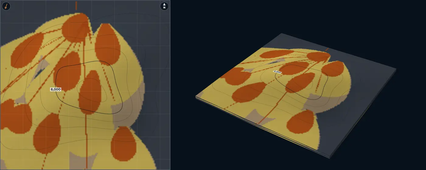
- Channel axis
- Lobe axis
- Channel margin
- Lobe off-axis
- Lobe fringe
- Levee and overbank
- Mudstone and shale
| Size | Default | Published | From |
|---|---|---|---|
| Lobe length | 4.97 mi8 km | 1.24 to 8.7 mi2 to 14 km | Deptuck et al. (2008); Prélat et al. (2010) |
| Lobe width | 3.11 mi5 km | 0.62 to 6.21 mi1 to 10 km | Deptuck et al. (2008); Prélat et al. (2010) |
| Lobe thickness | 98 ft30 m | 9.8 to 140 ft3 to 42 m | Deptuck et al. (2008); Prélat et al. (2010) |
| Feeder channel width | 655 ft200 m | 330 to 3,280 ft100 to 1,000 m | Cullis et al. (2018); Cullis et al. (2019) |
| Feeder channel thickness | 16 ft5 m | 3.3 to 98 ft1 to 30 m | Cullis et al. (2018) |
| Compensation offset | 2.49 mi4 km | 1.86 to 3.11 mi3 to 5 km | Deptuck et al. (2008); Cullis et al. (2018); Prélat, Hodgson and Flint (2009) |
| Paleoflow spread | 15° | Lab setting, no compiled range | – |
| Length / width | 1.6 | 1 to 3 | Deptuck et al. (2008) |
| Lobe width / thickness | 166.7 | 150 to 1,000 | Deptuck et al. (2008) |
| Feeder width / thickness | 40 | 10 to 100 | Shumaker et al. (2018); Cullis et al. (2019) |
Sources for this architecture
Deptuck et al. (2008)
Deptuck, M. E., Piper, D. J. W., Savoye, B., and Gervais, A., 2008, Dimensions and architecture of late Pleistocene submarine lobes off the northern margin of East Corsica: Sedimentology, v. 55, no. 4, p. 869–898. doi:10.1111/j.1365-3091.2007.00926.x (opens in a new tab)
Cullis et al. (2018)
Cullis, S., Colombera, L., Patacci, M., and McCaffrey, W. D., 2018, Hierarchical classifications of the sedimentary architecture of deep-marine depositional systems: Earth-Science Reviews, v. 179, p. 38–71. doi:10.1016/j.earscirev.2018.01.016 (opens in a new tab)
Prélat, Hodgson and Flint (2009)
Prélat, A., Hodgson, D. M., and Flint, S. S., 2009, Evolution, architecture and hierarchy of distributary deep-water deposits: a high-resolution outcrop investigation from the Permian Karoo Basin, South Africa: Sedimentology, v. 56, no. 7, p. 2132–2154. doi:10.1111/j.1365-3091.2009.01073.x (opens in a new tab)
Prélat et al. (2010)
Prélat, A., Covault, J. A., Hodgson, D. M., Fildani, A., and Flint, S. S., 2010, Intrinsic controls on the range of volumes, morphologies, and dimensions of submarine lobes: Sedimentary Geology, v. 232, no. 1–2, p. 66–76. doi:10.1016/j.sedgeo.2010.09.010 (opens in a new tab)
Straub et al. (2009)
Straub, K. M., Paola, C., Mohrig, D., Wolinsky, M. A., and George, T., 2009, Compensational stacking of channelized sedimentary deposits: Journal of Sedimentary Research, v. 79, no. 9, p. 673–688. doi:10.2110/jsr.2009.070 (opens in a new tab)
Cullis et al. (2019)
Cullis, S., Patacci, M., Colombera, L., Bührig, L., and McCaffrey, W. D., 2019, A database solution for the quantitative characterisation and comparison of deep-marine siliciclastic depositional systems: Marine and Petroleum Geology, v. 102, p. 321–339. doi:10.1016/j.marpetgeo.2018.12.023 (opens in a new tab)
Shumaker et al. (2018)
Shumaker, L. E., Jobe, Z. R., Johnstone, S. A., Pettinga, L. A., Cai, D., and Moody, J. D., 2018, Controls on submarine channel-modifying processes identified through morphometric scaling relationships: Geosphere, v. 14, no. 5, p. 2171–2187. doi:10.1130/GES01674.1 (opens in a new tab)
Amalgamated lobes Deepwater Unconfined basin-floor lobes, amalgamated
Geometry
On low-relief basin floors, such as the Tanqua Karoo, Amazon and Zaïre systems, lobes are areally extensive but thin: on average 8.7 mi14 km wide, 21.7 mi35 km long and 39 ft12 m thick, against 3.11 mi5 km by 4.97 mi8 km by 98 ft30 m where relief confines them; both kinds hold similar volumes, of the order of 0.24 to 0.48 mi³1 to 2 km³ (Prélat et al. 2010). In the Karoo, lobes are built of lobe elements and stack compensationally within a lobe complex on a 3.11 mi5 km scale (Prélat et al. 2009). A 7.46 mi12 km block sits inside one lobe’s medial reach, with the feeder off the block up-flow.
Facies
Lobe axis, off-axis and fringe in broad arcs across the block, proximal up-flow and distal down-flow. With little mud left between successive lobes, they amalgamate. The lab counts the lobe axis 88% net, off-axis 66% and fringe 35%.
NTG behaviour
High and well connected: wells kilometres apart read much the same, and NTG falls slowly down-flow and toward the lateral fringes.
Modern analogue
Amazon and Zaïre fans. Two of the low-relief systems whose channel-mouth lobes set the unconfined average (Prélat et al. 2010); the largest lobes there average 0.79 mi³3.3 km³.
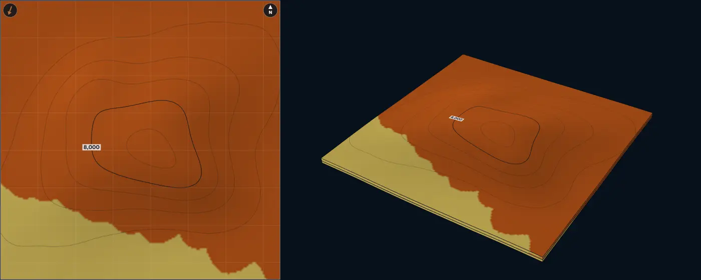
- Lobe axis
- Lobe off-axis
- Lobe fringe
- Mudstone and shale
| Size | Default | Published | From |
|---|---|---|---|
| Lobe length | 21.7 mi35 km | 4.97 to 21.7 mi8 to 35 km | Prélat et al. (2010) |
| Lobe width | 8.7 mi14 km | 3.11 to 8.7 mi5 to 14 km | Prélat et al. (2010) |
| Lobe thickness | 39 ft12 m | 9.8 to 140 ft3 to 42 m | Prélat et al. (2010); Deptuck et al. (2008) |
| Compensation offset | 3.11 mi5 km | 1.86 to 3.11 mi3 to 5 km | Prélat, Hodgson and Flint (2009); Deptuck et al. (2008) |
| Paleoflow spread | 8° | Lab setting, no compiled range | – |
| Length / width | 2.5 | 1 to 3 | Deptuck et al. (2008); Prélat et al. (2010) |
| Lobe width / thickness | 1,166.7 | 150 to 1,200 | Deptuck et al. (2008); Prélat et al. (2010) |
Sources for this architecture
Prélat et al. (2010)
Prélat, A., Covault, J. A., Hodgson, D. M., Fildani, A., and Flint, S. S., 2010, Intrinsic controls on the range of volumes, morphologies, and dimensions of submarine lobes: Sedimentary Geology, v. 232, no. 1–2, p. 66–76. doi:10.1016/j.sedgeo.2010.09.010 (opens in a new tab)
Prélat, Hodgson and Flint (2009)
Prélat, A., Hodgson, D. M., and Flint, S. S., 2009, Evolution, architecture and hierarchy of distributary deep-water deposits: a high-resolution outcrop investigation from the Permian Karoo Basin, South Africa: Sedimentology, v. 56, no. 7, p. 2132–2154. doi:10.1111/j.1365-3091.2009.01073.x (opens in a new tab)
Deptuck et al. (2008)
Deptuck, M. E., Piper, D. J. W., Savoye, B., and Gervais, A., 2008, Dimensions and architecture of late Pleistocene submarine lobes off the northern margin of East Corsica: Sedimentology, v. 55, no. 4, p. 869–898. doi:10.1111/j.1365-3091.2007.00926.x (opens in a new tab)
Frontal splays and terminal lobes Deepwater Distributary splays ending in terminal lobes
Geometry
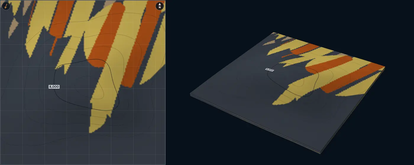
Where a leveed channel’s levees fade, it feeds frontal splays: low-sinuosity distributary-channel complexes that form lobate bodies up to 3.11 to 6.21 mi5 to 10 km wide and tens of kilometres long, reaching the distal edge of the system (Posamentier and Kolla 2003). Each splay here ends in a terminal lobe, and successive splays step aside.
Facies
Shallow distributary channel fills, lobe axis, off-axis, a broad lateral fringe and a narrow frontal fringe. In Fan 4 of the Karoo, frontal fringes are rich in hybrid beds and pass from thick-bedded sandstone over 0.62 to 1.24 mi1 to 2 km, while lateral fringes are ripple-laminated sandstone and siltstone that pass to the axis over several kilometres (Spychala et al. 2017). The lab counts the channels 90% net, lobe axis 88%, off-axis 66%, lateral fringe 35% and frontal fringe 30%.
NTG behaviour
Long sandy tongues aligned with the flow: wells along a splay agree, wells across it lose sand gradually into the lateral fringe, and the sand ends quickly at the front.
Analogue
Fan 4, Skoorsteenberg Formation, Karoo Basin. Compensationally stacked lobe complexes over an 309 mi²800 km² study area, their frontal and lateral fringes traced in outcrop and core (Spychala et al. 2017). Recent Amazon Fan. Its channel-mouth lobe complex, long the missing piece of the fan (Jegou et al. 2008).
- Distributary channel
- Lobe axis
- Lobe off-axis
- Lobe fringe
- Frontal fringe, hybrid beds
- Mudstone and shale
| Size | Default | Published | From |
|---|---|---|---|
| Splay width | 4.97 mi8 km | up to 6.21 mi10 km | Posamentier and Kolla (2003) |
| Splay length | 15.5 mi25 km | 6.21 to 55.9 mi10 to 90 km | Posamentier and Kolla (2003) |
| Splay thickness | 20 ft6 m | Lab setting, no compiled range | – |
| Frontal-fringe length | 0.93 mi1.5 km | 0.62 to 1.24 mi1 to 2 km | Spychala et al. (2017) |
| Lateral-fringe width | 1.24 mi2 km | 1.24 to 3.11 mi2 to 5 km | Spychala et al. (2017) |
| Distributary channel width | 490 ft150 m | Lab setting, no compiled range | – |
| Paleoflow spread | 10° | Lab setting, no compiled range | – |
Sources for this architecture
Posamentier and Kolla (2003)
Posamentier, H. W., and Kolla, V., 2003, Seismic Geomorphology and Stratigraphy of Depositional Elements in Deep-Water Settings: Journal of Sedimentary Research, v. 73, no. 3, p. 367–388. doi:10.1306/111302730367 (opens in a new tab)
Spychala et al. (2017)
Spychala, Y. T., Hodgson, D. M., Prélat, A., Kane, I. A., Flint, S. S., and Mountney, N. P., 2017, Frontal and Lateral Submarine Lobe Fringes: Comparing Sedimentary Facies, Architecture and Flow Processes: Journal of Sedimentary Research, v. 87, no. 1, p. 75–96. doi:10.2110/jsr.2017.2 (opens in a new tab)
Jegou et al. (2008)
Jegou, I., Savoye, B., Pirmez, C., and Droz, L., 2008, Channel-mouth lobe complex of the recent Amazon Fan: The missing piece: Marine Geology, v. 252, no. 1–2, p. 62–77. doi:10.1016/j.margeo.2008.03.004 (opens in a new tab)
Other
Reef and shoal Carbonate Rimmed platform margin: reef rim, shoals, lagoon, talus
Geometry
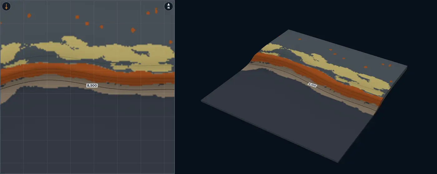
A reef rim at the platform margin, grainstone shoals behind it, patch reefs in the lagoon and talus down the slope. Mapped facies patches on Pacific reefs run from the 43,594 ft²4,050 m² mapping limit to 39 mi²100 km², small patches far outnumbering large ones, and patches over 0.39 mi²1 km² tend to be narrow and elongate along the shelf (Purkis et al. 2007). The lab’s patch-reef range, 230 to 3,705 ft70 to 1,130 m across, is the equal-area diameter of patches from that limit to 0.39 mi²1 km². Ooid shoals form bars up to several kilometres in wavelength and several metres high (Rankey et al. 2006); on Great Bahama Bank tidal sand bodies range from narrow bars split by wide, deep channels to broader, irregular bars with narrow channels (Harris et al. 2011). No compiled width was found for the reef rim, so rim width and segment length are lab settings.
Facies
Reef core, grainstone shoal, reef talus and slope apron, lagoon mud. On ooid bars the best-sorted, coarsest grains sit on the crests and the finest in the deeper interior and on the flanks (Rankey et al. 2006). The lab counts reef core 82% net, shoal 74%, talus 42% and lagoon mud 6%.
NTG behaviour
Net here means reservoir-quality carbonate. It is high on the rim and the shoals and falls to lagoon mud within a few kilometres inboard, so a well on the rim says little about the lagoon. Among Bahamian tidal shoals, the widest oolitic belts also have the tallest bars (Rankey and Reeder 2011).
Modern analogue
Great Bahama Bank. The sand belt rimming the southern end of the Tongue of the Ocean and the Schooners shoals at the north end of Exuma Sound (Harris et al. 2011), and Lily Bank, a tide-dominated ooid shoal (Rankey et al. 2006).
- Reef core
- Grainstone shoal
- Reef talus and slope apron
- Lagoon mud
- Mudstone and shale
| Size | Default | Published | From |
|---|---|---|---|
| Reef-rim width | 1,970 ft600 m | Lab setting, no compiled range | – |
| Reef segment length | 1.55 mi2.5 km | Lab setting, no compiled range | – |
| Patch-reef diameter | 985 ft300 m | 230 to 3,705 ft70 to 1,130 m | Purkis et al. (2007) |
| Shoal length | 1.55 mi2.5 km | up to 3.11 mi5 km | Rankey et al. (2006); Harris et al. (2011) |
| Shoal width | 2,625 ft800 m | Lab setting, no compiled range | – |
| Shoal thickness | 13 ft4 m | up to 16 ft5 m | Rankey et al. (2006) |
Sources for this architecture
Purkis et al. (2007)
Purkis, S. J., Kohler, K. E., Riegl, B. M., and Rohmann, S. O., 2007, The statistics of natural shapes in modern coral reef landscapes: The Journal of Geology, v. 115, no. 5, p. 493–508. doi:10.1086/519774 (opens in a new tab)
Rankey et al. (2006)
Rankey, E. C., Riegl, B., and Steffen, K., 2006, Form, function and feedbacks in a tidally dominated ooid shoal, Bahamas: Sedimentology, v. 53, no. 6, p. 1191–1210. doi:10.1111/j.1365-3091.2006.00807.x (opens in a new tab)
Harris et al. (2011)
Harris, P. M., Purkis, S. J., and Ellis, J., 2011, Analyzing spatial patterns in modern carbonate sand bodies from Great Bahama Bank: Journal of Sedimentary Research, v. 81, no. 3, p. 185–206. doi:10.2110/jsr.2011.21 (opens in a new tab)
Rankey and Reeder (2011)
Rankey, E. C., and Reeder, S. L., 2011, Holocene oolitic marine sand complexes of the Bahamas: Journal of Sedimentary Research, v. 81, no. 2, p. 97–117. doi:10.2110/jsr.2011.10 (opens in a new tab)
Aeolian dunes Aeolian Dune sets and interdunes across an erg
Geometry
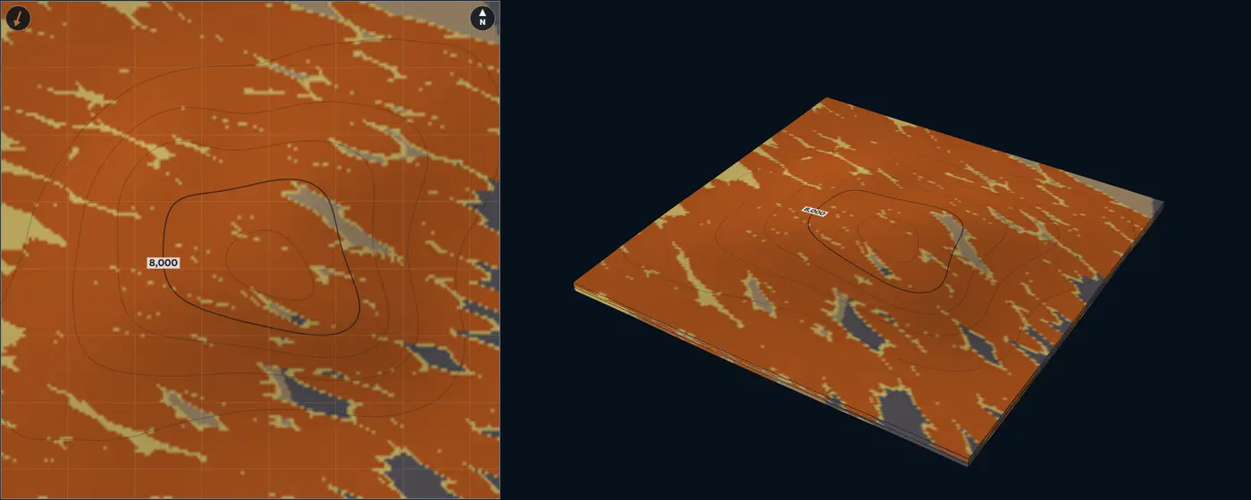
Cross-bedded dune sets stack where bedforms climb, separated by interdune deposits; the block runs from a dry erg centre on one side to a wet erg margin on the other. In the Etjo Formation, Namibia, the thickest preserved sets fall from 170 ft52 m in the basin depocentre to 26 ft8 m at its margin, because the bedforms climbed at lower angles there, not because they were smaller; interdune surfaces form troughs 1,640 ft500 m wide across the wind (Mountney and Howell 2000). Interdune deposits form flat, laterally discontinuous lenses across the wind (Kocurek 1981). Across 56 aeolian systems, foreland basins preserve thick dune sets, intracratonic and rift basins thin ones (Cosgrove et al. 2023).
Facies
Dune sets of grainflow and wind-ripple strata, dune toesets and dry interdunes, damp and wet interdunes, playa and sabkha mud. Toward the erg margin, interdunes change from isolated dry hollows to interconnected damp and wet ponds, then to fluvially flooded corridors (Mountney and Jagger 2004), and one interdune can pass from wet through damp to dry (Mountney and Thompson 2002). The lab counts dune sets 95% net, toesets and dry interdunes 70%, damp and wet interdunes 30% and playa mud 5%.
NTG behaviour
Very high in the erg centre, where dune sets amalgamate. Toward the margin, wet interdunes and playa mud split the sand, and low-permeability interdune units can act as baffles or barriers to flow (Mountney 2012).
Modern analogue
White Sands, New Mexico. A simple dune field, with one population of dune spacings and crest lengths (Ewing et al. 2006). Etjo Formation, northwest Namibia. A Cretaceous erg whose sets and bounding surfaces record the original bedforms (Mountney and Howell 2000).
- Dune set
- Dune toeset and dry interdune
- Damp and wet interdune
- Playa and sabkha mud
| Size | Default | Published | From |
|---|---|---|---|
| Dune-set thickness | 66 ft20 m | 26 to 170 ft8 to 52 m | Mountney and Howell (2000) |
| Interdune width | 1,640 ft500 m | One documented example, 1,640 ft500 m | Mountney and Howell (2000) |
| Dune spacing | 2,955 ft900 m | Lab setting, no compiled range | – |
| Crest length | 1.86 mi3 km | Lab setting, no compiled range | – |
| Wind-direction spread | 10° | Lab setting, no compiled range | – |
Sources for this architecture
Mountney and Howell (2000)
Mountney, N. P., and Howell, J. A., 2000, Aeolian architecture, bedform climbing and preservation space in the Cretaceous Etjo Formation, NW Namibia: Sedimentology, v. 47, no. 4, p. 825–849. doi:10.1046/j.1365-3091.2000.00318.x (opens in a new tab)
Kocurek (1981)
Kocurek, G., 1981, Significance of interdune deposits and bounding surfaces in aeolian dune sands: Sedimentology, v. 28, no. 6, p. 753–780. doi:10.1111/j.1365-3091.1981.tb01941.x (opens in a new tab)
Cosgrove et al. (2023)
Cosgrove, G. I. E., Colombera, L., and Mountney, N. P., 2023, Quantitative analysis of aeolian stratigraphic architectures preserved in different tectonic settings: Earth-Science Reviews, v. 237, p. 104293. doi:10.1016/j.earscirev.2022.104293 (opens in a new tab)
Mountney and Jagger (2004)
Mountney, N. P., and Jagger, A., 2004, Stratigraphic evolution of an aeolian erg margin system: the Permian Cedar Mesa Sandstone, SE Utah, USA: Sedimentology, v. 51, no. 4, p. 713–743. doi:10.1111/j.1365-3091.2004.00646.x (opens in a new tab)
Mountney and Thompson (2002)
Mountney, N. P., and Thompson, D. B., 2002, Stratigraphic evolution and preservation of aeolian dune and damp/wet interdune strata: an example from the Triassic Helsby Sandstone Formation, Cheshire Basin, UK: Sedimentology, v. 49, no. 4, p. 805–833. doi:10.1046/j.1365-3091.2002.00472.x (opens in a new tab)
Mountney (2012)
Mountney, N. P., 2012, A stratigraphic model to account for complexity in aeolian dune and interdune successions: Sedimentology, v. 59, no. 3, p. 964–989. doi:10.1111/j.1365-3091.2011.01287.x (opens in a new tab)
Ewing et al. (2006)
Ewing, R. C., Kocurek, G., and Lake, L. W., 2006, Pattern analysis of dune-field parameters: Earth Surface Processes and Landforms, v. 31, no. 9, p. 1176–1191. doi:10.1002/esp.1312 (opens in a new tab)
Lacustrine fan delta Lacustrine Gilbert-type fan deltas on a lake margin
Geometry
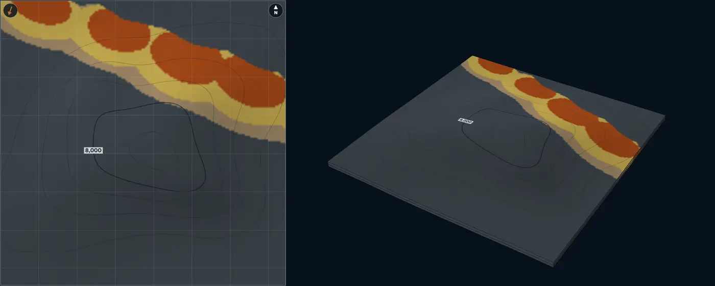
Fan deltas build out from the lake margin, here a fault-bounded edge on the up-flow side of the block. In rift basins, footwall-derived coarse-grained deltas are generally Gilbert-type, isolated fan- to wedge-shaped bodies of less than 3.86 mi²10 km² (Gawthorpe and Colella 1990). Gilbert-type deltas range from 6.6 to 2,135 ft2 to 650 m thick, and their thickness scales with their length (Budai et al. 2021).
Facies
Topset (braided-plain gravel and sand), steep foreset (avalanche gravel and sand), bottomset (turbidites and heterolithics), lake mud. The topset meets the foreset at a sharp brink; the foreset grades into the bottomset. Gilbert-type deltas fall into gravel- and sand-dominated types with contrasting topset, foreset and bottomset facies (Budai et al. 2021); a delta’s character depends first on its plain, front, slope and prodelta, and second on its feeder (Postma 1990). The lab counts the topset 85% net, foreset 75% and bottomset 35%.
NTG behaviour
Sand stays in a belt along the lake margin and coarsens up in every column as the deltas build out; farther out NTG drops to lake mud.
Modern analogue
South Rukuru fan delta, Lake Malawi. A large fan delta and sub-lacustrine fan on a border-fault margin, with sand-dominated facies in more than 1,970 ft600 m of water (Soreghan et al. 1999). Kulu Formation, Rusinga Island, Lake Victoria. A Miocene Gilbert-type fan delta with classic topset, foreset and bottomset, shed from a horst about 3.11 mi5 km long (Bestland 1991).
- Fan-delta topset
- Fan-delta foreset
- Fan-delta bottomset
- Lacustrine mudstone
| Size | Default | Published | From |
|---|---|---|---|
| Fan-delta area | 1.93 mi²5 km² | up to 3.86 mi²10 km² | Gawthorpe and Colella (1990) |
| Fan-delta thickness | 120 ft36 m | 6.6 to 2,135 ft2 to 650 m | Budai et al. (2021) |
| Fan-delta spacing | 2.49 mi4 km | Lab setting, no compiled range | – |
| Progradation | 0.93 mi1.5 km | Lab setting, no compiled range | – |
| Paleoflow spread | 10° | Lab setting, no compiled range | – |
Sources for this architecture
Gawthorpe and Colella (1990)
Gawthorpe, R. L., and Colella, A., 1990, Tectonic Controls on Coarse-Grained Delta Depositional Systems in Rift Basins: in Coarse-Grained Deltas: International Association of Sedimentologists Special Publication 10, p. 113–127. doi:10.1002/9781444303858.ch6 (opens in a new tab)
Budai et al. (2021)
Budai, S., Colombera, L., and Mountney, N. P., 2021, Quantitative characterization of the sedimentary architecture of Gilbert-type deltas: Sedimentary Geology, v. 426, p. 106022. doi:10.1016/j.sedgeo.2021.106022 (opens in a new tab)
Postma (1990)
Postma, G., 1990, Depositional Architecture and Facies of River and Fan Deltas: A Synthesis: in Coarse-Grained Deltas: International Association of Sedimentologists Special Publication 10, p. 13–27. doi:10.1002/9781444303858.ch2 (opens in a new tab)
Soreghan et al. (1999)
Soreghan, M. J., Scholz, C. A., and Wells, J. T., 1999, Coarse-grained, deep-water sedimentation along a border fault margin of Lake Malawi, Africa; seismic stratigraphic analysis: Journal of Sedimentary Research, v. 69, no. 4, p. 832–846. doi:10.2110/jsr.69.832 (opens in a new tab)
Bestland (1991)
Bestland, E. A., 1991, A Miocene Gilbert-type fan-delta from a volcanically influenced lacustrine basin, Rusinga Island, Lake Victoria, Kenya: Journal of the Geological Society, v. 148, no. 6, p. 1067–1078. doi:10.1144/gsjgs.148.6.1067 (opens in a new tab)
Try this
One well, many answers. W1 at 78% leaves several architectures in play.
Spacing tells them apart. Nine rich wells 1.9 mi3 km apart: widespread sands, the amalgamated lobes and the aeolian dunes, rank first; the confined channel falls far behind.
A line of sand. Rich wells along the paleoflow, poor ones beside them: the confined channel ranks first.
The turtle's crest. The inverted mini-basin's crest holds the ponded sand.
A fault that steers. Lobes thicken and stretch along a growing fault.
Eroded out. W2 sits where zone 1 is cut away; only zone 2 counts.
About the lab
Map it to your field
Sketch your well spacing on the grid: one square is 0.6 mi1 km. Turn on Place wells and click each well where it sits relative to the others, then drag it or type its position. Type each well's NTG per zone, and leave a zone blank where the well stops short. Set up to eight zones and their thicknesses, and switch any zone to Shale for a persistent, non-reservoir interval between your sands: it stays mudstone across the block, keeps its thickness and is left out of the fit. Pick the trap closest to yours, then compare which architectures fit and where they disagree.
The eight traps
- Anticline. An irregular four-way closure. When it grew during deposition, the zones thin over the crest.
- Tilted fault block. A rotated block whose crest seals against a normal fault. A syndepositional fault thickens the hanging wall and turns flow along it.
- Salt mini-basin. A bowl between salt walls. Fill thickens to the centre; traps sit where beds turn up against the salt.
- Unconformity trap. Tilted zones cut by erosion, each sealed where it subcrops updip.
- Turtle structure. An inverted mini-basin: the thickest, best-ponded sand now sits on the crest.
- Horst and graben. A raised rift block between two grabens, which fill thick when the faults move during deposition.
- Growth fault and rollover. A deltaic fault whose hanging wall thickens into it and rolls over into an anticline.
- Carbonate platform margin. A platform edge with a reef rim, thick on the platform and thin in the basin. Pair it with Reef and shoal.
How it works
Each architecture is built from objects at published sizes: sinuous channels with levees, lobes with their feeder and distributary channels, mouth bars at the tips of distributaries on a delta-front lobe, reefs and shoals, laid down one after another inside each zone until it holds its share of sand. Open Element dimensions to change those sizes. Where a well has too little sand, the lab adds an object through it; where it has too much, it moves the object that put it there. A short-range correction then makes every typed value exact.
In the 3D block, Slice cuts it along an Inline (north to south), a Crossline (east to west), a Depth slice or an Arb line turned in 5-degree steps, and shows the facies on the cut face; Flip shows the other side. The faces are read from the same columns as the map and the wells, and the map draws the trace of the line.
The fit ranks how readily each architecture, left to itself, produces your numbers: each well on its own, and every pair of wells within 1.9 mi3 km together. The pairs are what tell a narrow channel from a wide lobe. The drill-here map repeats the whole conditioned build with new seeds and counts, at every spot, how often the NTG lands in your target range. The same settings always give the same pictures, so a shared link redraws exactly what you saw.
The method in more detail
A zone is 32 levels thick. Every object occupies a span of levels at each point it covers. Channels are erosive: their fills replace what they cut, so they cut into the lobes below them. Lobes, bars, reefs and shoals are depositional: where a younger one overlaps an older deposit in the same level, it can raise that level's sand but never replace the older sand with its own muddier fringe. A bed thinner than a level still takes one level at its core. A cell's NTG is the mean sand fraction of its levels: a channel-axis level counts 93%, a levee level 28% (thin-bedded sand in a muddy element), mudstone 2%. Inside a lobe, a mouth bar or a shoreface, and from a channel’s axis to its margin, the facies grade into one another across a transition band (a lab choice: the sources describe the change as progressive but give no cut-off), so NTG changes gradually; the erosional edge of a channel fill against its host stays sharp. The overall sand content of a zone is drawn from the architecture's range and pulled toward the average of your wells, more strongly as you add wells.
When the structure grew during deposition, flows feel it: they steer down the paleo-slope, run along an active fault or salt wall, and pond in the lows, while reefs favour the highs. When it formed later, deposition ignores it and the layers are simply folded or offset.
The fit is a pairwise composite likelihood over 60 unconditioned realizations of each architecture, with equal prior weight on all 19, each using its own element dimensions. It is shown against the best fit, as how many times less readily each architecture produces your values, with words on Kass and Raftery's Bayes-factor steps: within 3 times the best it fits, 3 to 20 times is possible, 20 to 150 unlikely, beyond that very unlikely. A pairwise likelihood counts each well more than once, so it grows confident faster than a full one would: read it as a ranking, not a probability. A value is flagged as rare when none of those 60 realizations comes within 7.5 points of it at that spot.
Sources for this section
Deutsch and Wang (1996)
Deutsch, C. V., and Wang, L., 1996, Hierarchical object-based stochastic modeling of fluvial reservoirs: Mathematical Geology, v. 28, no. 7, p. 857–880. doi:10.1007/BF02066005 (opens in a new tab)
Kass and Raftery (1995)
Kass, R. E., and Raftery, A. E., 1995, Bayes factors: Journal of the American Statistical Association, v. 90, no. 430, p. 773–795. doi:10.1080/01621459.1995.10476572 (opens in a new tab)
Holden et al. (1998)
Holden, L., Hauge, R., Skare, Ø., and Skorstad, A., 1998, Modeling of fluvial reservoirs with object models: Mathematical Geology, v. 30, no. 5, p. 473–496. doi:10.1023/A:1021769526425 (opens in a new tab)
Journel (1974)
Journel, A. G., 1974, Geostatistics for conditional simulation of ore bodies: Economic Geology, v. 69, no. 5, p. 673–687. doi:10.2113/gsecongeo.69.5.673 (opens in a new tab)
Why the architecture matters
NTG is a ratio over a column. It says nothing about the shape of the sand around it. In channelized models, connectivity falls away sharply as NTG drops, and how sharply depends on the architecture. Lobes stack where the last lobe left a low, so their sand shifts sideways from one zone to the next. And NTG itself depends on the cutoffs used to call rock net.
Sources for this section
Larue and Hovadik (2006)
Larue, D. K., and Hovadik, J., 2006, Connectivity of channelized reservoirs: a modelling approach: Petroleum Geoscience, v. 12, no. 4, p. 291–308. doi:10.1144/1354-079306-699 (opens in a new tab)
McHargue et al. (2011)
McHargue, T., Pyrcz, M. J., Sullivan, M. D., Clark, J. D., Fildani, A., Romans, B. W., Covault, J. A., Levy, M., Posamentier, H. W., and Drinkwater, N. J., 2011, Architecture of turbidite channel systems on the continental slope: patterns and predictions: Marine and Petroleum Geology, v. 28, no. 3, p. 728–743. doi:10.1016/j.marpetgeo.2010.07.008 (opens in a new tab)
Prélat, Hodgson and Flint (2009)
Prélat, A., Hodgson, D. M., and Flint, S. S., 2009, Evolution, architecture and hierarchy of distributary deep-water deposits: a high-resolution outcrop investigation from the Permian Karoo Basin, South Africa: Sedimentology, v. 56, no. 7, p. 2132–2154. doi:10.1111/j.1365-3091.2009.01073.x (opens in a new tab)
Straub et al. (2009)
Straub, K. M., Paola, C., Mohrig, D., Wolinsky, M. A., and George, T., 2009, Compensational stacking of channelized sedimentary deposits: Journal of Sedimentary Research, v. 79, no. 9, p. 673–688. doi:10.2110/jsr.2009.070 (opens in a new tab)
Worthington and Cosentino (2005)
Worthington, P. F., and Cosentino, L., 2005, The role of cutoffs in integrated reservoir studies: SPE Reservoir Evaluation & Engineering, v. 8, no. 4, p. 276–290. doi:10.2118/84387-PA (opens in a new tab)
What it simplifies
- One 7.5 mi12 km block. Element sizes come from published compilations and modern analogues, not from any one basin; reef-rim width and segment length, shoal width, delta-lobe length and paleoflow spread are lab settings, as no compiled range was found.
- NTG is a single number per zone at each well, with no cutoff, log or core behind it.
- Facies are painted, not grown from flow: no grain size, no compaction, no diagenesis.
- Faults are vertical steps, and timing is all or nothing: growth either happened during deposition or after it.